Filtering

Apply filters to neural signals, including highpass, lowpass, bandpass & bandstop filters.

This tutorial primarily covers the neurodsp.filt module.

Filtering with NeuroDSP

The filter_signal() function is the main function for filtering using NeuroDSP.

In this tutorial, we will examine filtering signals with different passbands. The passband of a filter is the range of frequencies that can ‘pass’ through a filter.

The following articles also have additional information on filtering electrophysiological data:

• Widman et al., 2015

• de Cheveigne & Nelken, 2019

# Import filter function
from neurodsp.filt import filter_signal

# Import simulation code for creating test data
from neurodsp.sim import sim_combined
from neurodsp.utils import set_random_seed, create_times

# Import utilities for loading and plotting data
from neurodsp.utils.download import load_ndsp_data
from neurodsp.plts.time_series import plot_time_series

# Set the random seed, for consistency simulating data
set_random_seed(0)

# General settings for simulations
fs = 1000
n_seconds = 5

# Set the default aperiodic exponent
exp = -1

# Generate a times vector, for plotting
times = create_times(n_seconds, fs)

Bandpass filters

A bandpass filter allows through frequencies within a given frequency range.

These filters can be useful to filter a signal to a specific band range, for example filtering to the theta range, defined as 4-8 Hz.

# Set the frequency in our simulated signal
freq = 6

# Set up simulation for a signal with aperiodic activity and an oscillation
components = {'sim_powerlaw' : {'exponent' : exp},
              'sim_oscillation' : {'freq' : 6}}
variances = [0.1, 1]

# Simulate our signal
sig = sim_combined(n_seconds, fs, components, variances)

# Define a frequency range to filter the data
f_range = (4, 8)

# Bandpass filter the data, across the band of interest
sig_filt = filter_signal(sig, fs, 'bandpass', f_range)

# Plot filtered signal
plot_time_series(times, [sig, sig_filt], ['Raw', 'Filtered'])

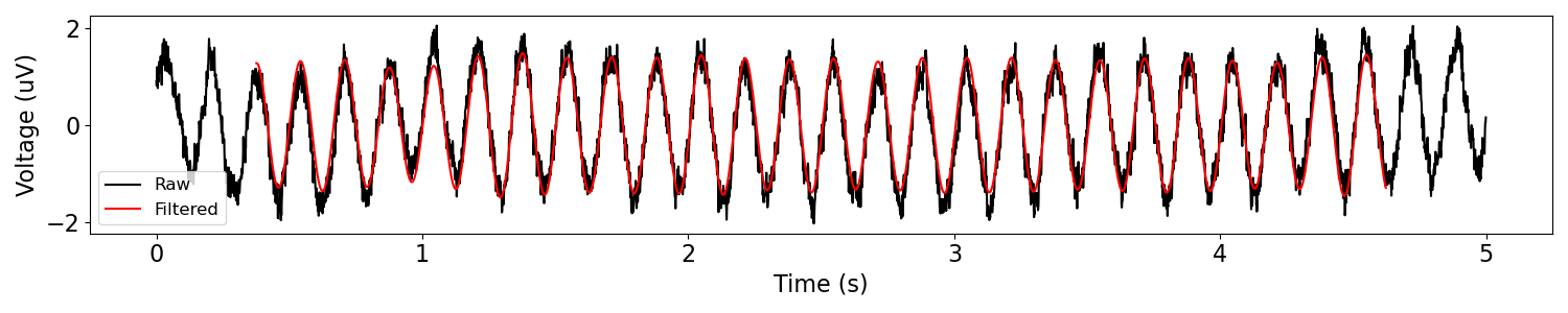
Notice that the edges of the filtered signal are clipped (no red).

Edge artifact removal is done by default in NeuroDSP filtering, because the signal samples at the edges only experienced part of the filter.

To bypass this feature, set remove_edges=False, but at your own risk!

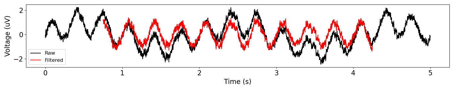
Highpass filter

Highpass filters are filters that pass through all frequencies above a specified cutoff point.

These filters can be used to remove low frequency drift from the data.

# Settings for the rhythmic components in the data
freq1 = 3
freq2 = 0.5

# Set up simulation for a signal with aperiodic activity, an oscillation, and low frequency drift
components = {'sim_powerlaw' : {'exponent' : exp},
              'sim_oscillation' : [{'freq' : freq1}, {'freq' : freq2}]}
variances = [0.1, 1, 1]

# Generate a signal including low-frequency activity
sig = sim_combined(n_seconds, fs, components, variances)

# Filter the data with a highpass filter
f_range = (2, None)
sig_filt = filter_signal(sig, fs, 'highpass', f_range)

# Plot filtered signal
plot_time_series(times, [sig, sig_filt], ['Raw', 'Filtered'])

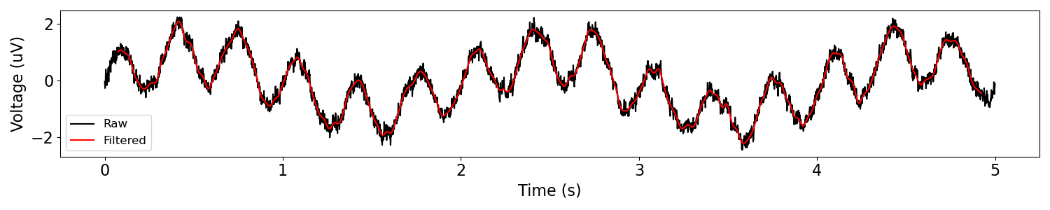
Lowpass filter

Lowpass filters are filters that pass through all frequencies below a specified cutoff point.

These filters can be used to remove high frequency activity from the data.

# Filter the data
f_range = (None, 20)
sig_filt = filter_signal(sig, fs, 'lowpass', f_range)

# Plot filtered signal
plot_time_series(times, [sig, sig_filt], ['Raw', 'Filtered'])

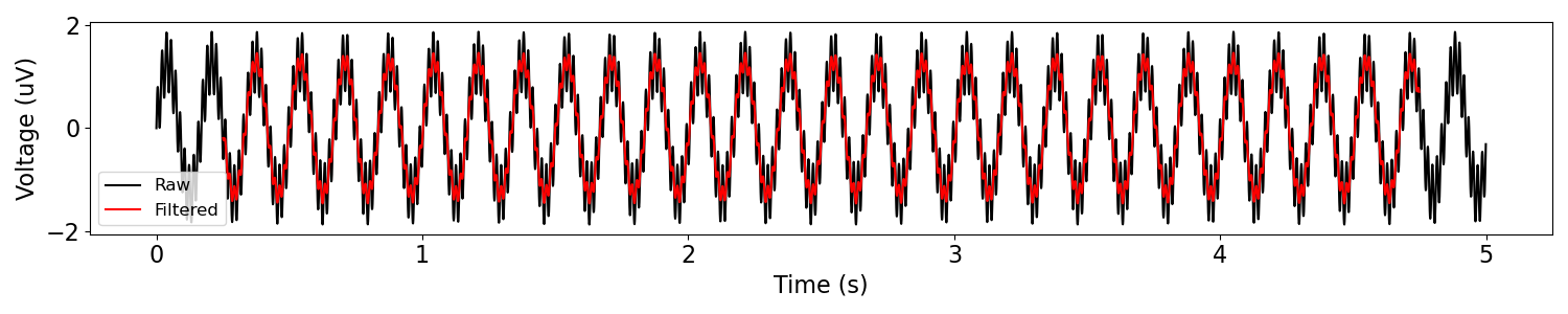
Bandstop filter

Bandstop filters are filters that remove a specified band range from the data.

Next let’s try a bandstop filter, to remove 60 Hz noise from the data.

Notice that it is necessary to set a non-default filter length because a filter of length 3 cycles of a 58Hz oscillation would not attenuate the 60Hz oscillation much (try this yourself!).

# Generate a signal, with a low frequency oscillation and 60 Hz line noise
components = {'sim_oscillation' : [{'freq' : 6}, {'freq' : 60}]}
variances = [1, 0.2]
sig = sim_combined(n_seconds, fs, components, variances)

# Filter the data
f_range = (58, 62)
sig_filt = filter_signal(sig, fs, 'bandstop', f_range, n_seconds=0.5)

/Users/tom/opt/anaconda3/envs/mne/lib/python3.8/site-packages/neurodsp/filt/checks.py:153: UserWarning: The filter attenuation never goes below -20 dB. Increase filter length.
  warn('The filter attenuation never goes below {} dB. '\

# Plot filtered signal
plot_time_series(times, [sig, sig_filt], ['Raw', 'Filtered'])

Real Data Example

Finally, let’s apply a filter to a segment of real data.

In this example, we will apply a bandpass filter in the beta range to a segment of neural data.

# Download, if needed, and load example data file
sig = load_ndsp_data('sample_data_1.npy', folder='data')

# Set sampling rate, and create a times vector for plotting
fs = 1000
times = create_times(len(sig)/fs, fs)

# Define the range to filter to data to
f_range = (13, 30)

# Filter the data
sig_filt = filter_signal(sig, fs, 'bandpass', f_range, n_cycles=3)

# Plot filtered signal
plot_time_series(times, [sig, sig_filt], ['Raw', 'Filtered'], xlim=[2, 5])

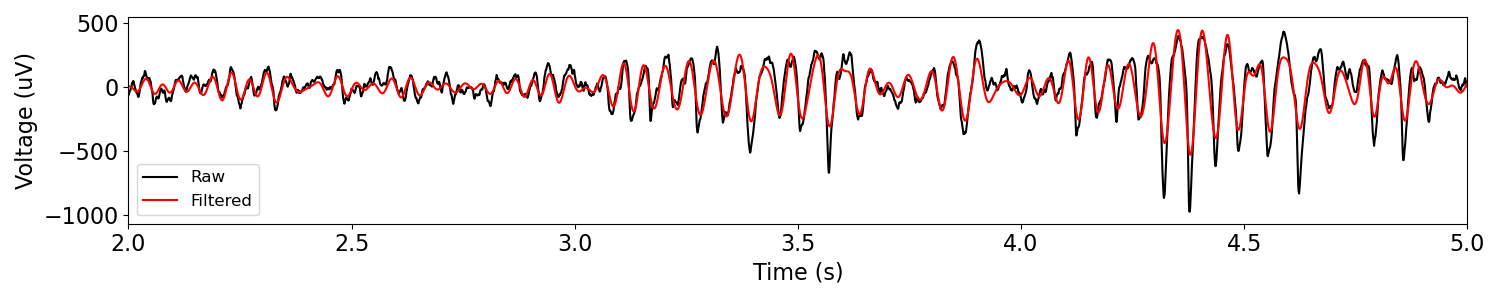
In the above, we can see the original and filtered versions of some real neural data.

You might notice that in the filtered time series, the resulting oscillation appears to be more sinusoidal than the original signal really is.

If you are interested in this problem, and how to deal with it, you should check out bycycle, which is a tool for time-domain analyses of waveform shape.

Conclusion

This tutorial has been a brief introduction to applying the filters that are available in NeuroDSP. Note that in practice you will likely do more checking of filters that you use (checking the filter response, for example), and may need to update settings.

For more information on different kinds of filters and their settings and properties, and how to evaluate filters see the subsequent tutorials.