FIR Filters

Design, apply, and evaluate FIR Filters.

This tutorial covers the design and application of Finite Impulse Response (FIR) filters, available in neurodsp.filt.fir.

# Import functions for simulating test data
from neurodsp.sim import sim_combined
from neurodsp.utils import set_random_seed, create_times

# Import functions for FIR filtering
from neurodsp.filt import filter_signal
from neurodsp.filt.fir import design_fir_filter, apply_fir_filter
from neurodsp.filt.utils import compute_frequency_response, compute_transition_band

# Import plotting functions
from neurodsp.plts import plot_filter_properties, plot_time_series

FIR Filters

Finite impulse response filters are filters for which the response to a single impulse is finite. FIR filters are common and useful, as they can be designed to have specified time-frequency resolution properties, which can be controlled by manipulating the filter length.

An impulse response is the output of the convolution of a short duration signal (i.e. Kronecker delta function) with the filter. FIR filtering involves convolving an input signal with the impulse response of the filter.

Each timepoint in the output signal is expressed as:

\[y(n) = \sum_{k=0}^M b_k x(n-k)\]

Where each output \(y(n)\) is the sum of the product of the filter coefficients (i.e. values from the impulse response, \(b_k\)) and past values of the input signal \(x(n-k)\). The filter order or the length of the impulse response minus one is represented by \(M\).

This formula also has a frequency representation:

\[H(z) = \sum_{k=0}^M b_k z^{-k}\]

The FIR filters available in NeuroDSP are designed using the window method, using ‘firwin’ from scipy, and applied by convolution. For more information on these implementations, see the scipy documentation.

Simulate an example signal to use for this example.

# Set the random seed, for consistency simulating data
set_random_seed(0)

# Define settings for simulating time series
n_seconds = 1
fs = 1000
components = {'sim_powerlaw' : {'exponent' : 0},
              'sim_oscillation' : {'freq' : 10}}
variances = [0.1, 1]

# Simulate time series, and create associated time definition
times = create_times(n_seconds, fs)
sig = sim_combined(n_seconds, fs, components, variances)

Design an FIR Filter

First, let’s design an FIR filter, which means to generate the filter coefficients that will instantiate our filter, which we can do with the design_fir_filter() function.

To do so, we need to define some filter settings, including the passband and cutoff frequencies.

We also need to specify the filter length, which can be defined either in seconds, or as a number of cycles (defined as the low cutoff frequency). The default filter length is 3 cycles. You may need to update this value to customize the filter length, as this impacts the frequency response.

# Define filter settings
pass_type = 'bandpass'
f_range = (8, 13)
n_cycles = 3

# Design the filter coefficients for a specified filter
filter_coefs = design_fir_filter(fs, pass_type, f_range, n_cycles=n_cycles)

Now that we have our filter coefficients, we can evaluate our filter.

Next, we can calculate the frequency response, \(b_k\), for our alpha bandpass filter.

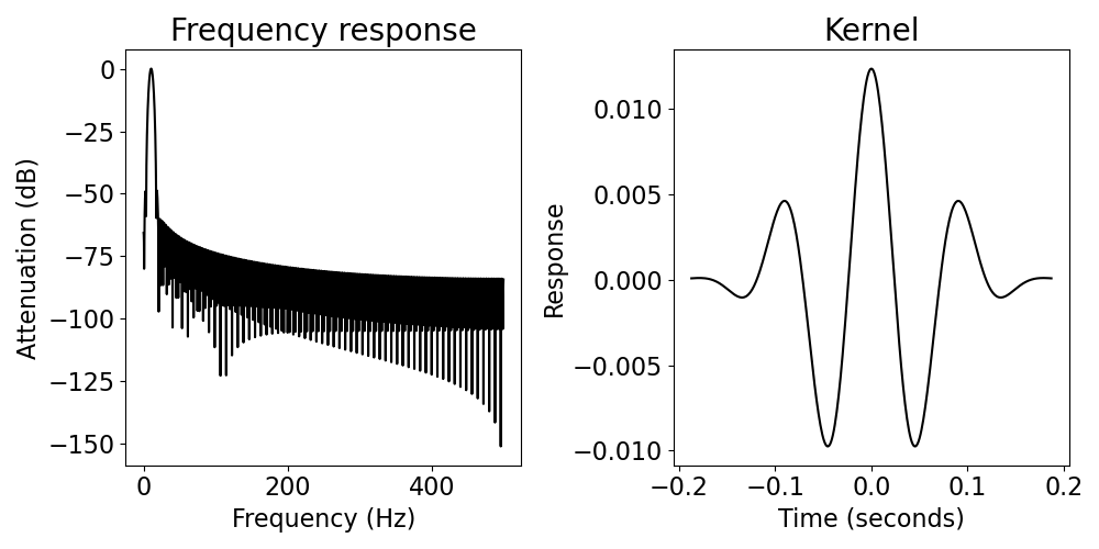
# Compute the frequency response of the filter
f_db, db = compute_frequency_response(filter_coefs, 1, fs)

# Plot the filter properties
plot_filter_properties(f_db, db, fs, filter_coefs)

On the right is the impulse response, or the filter kernel. This is a visualization of our filter coefficients, which also demonstrates the activity of our filter for a single point (the impulse response).

On the left, we can see the frequency response of our filter, which shows us how different frequencies are affected by our filter. Ideally, we want zero attenuation in our passband, and a lot of attenuation in the stopband(s).

Another way to quantify these properties is the transition band, which is bandwidth (in Hz) that it takes for the filter to change from high to low attenuation. This quantifies how sharp the transition is between stopband and passband. By default, transition bands are computed as the range between -20 dB and -3 dB attenuation, but you can also customize these values.

# Compute the transition band of the filter
t_band = compute_transition_band(f_db, db)

# Print the transition band
print('Transition band: {:4.2f}'.format(t_band))

Transition band: 3.00

In the above, we have designed and evaluated an FIR filter. Note that the properties of the filter will depend on the passband and cutoff frequencies, and especially the filter length.

You can explore changing these settings to see how they impact the filter properties.

Apply an FIR Filter

Next, we can apply our filter to the data. FIR filter can be applied to signals by convolution, which we can do with the apply_fir_filter() function.

# Apply the filter
sig_filt = apply_fir_filter(sig, filter_coefs)

# Plot the signal and filtered version
plot_time_series(times, [sig, sig_filt], ['Raw', 'Filtered'])

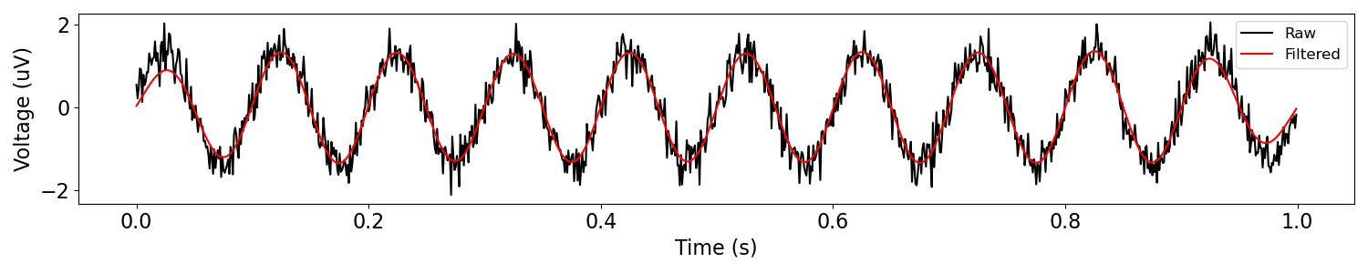
In the above, we can see both the original signal, and the filtered version.

Note that inspecting the filtered signal together with the original signal is recommended.

Using filter_signal

In the above, we did a step-by-step procedure of designing, evaluating, and applying our filter.

Note that all of these elements can also be done directly through the filter_signal() function.

# Filter our signal, using the main filter function, with extra options
sig_filt2, filter_kernel = filter_signal(sig, fs, pass_type, f_range,
                                         filter_type='fir', print_transitions=True,
                                         plot_properties=True, return_filter=True)

Transition bandwidth is 3.0 Hz.
Pass/stop bandwidth is 5.0 Hz.

# Plot the signal and filtered version
plot_time_series(times, [sig, sig_filt2], ['Raw', 'Filtered'])

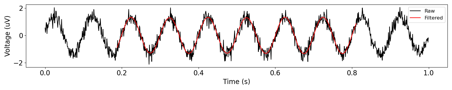
You might notice in the above plot, the edges of the filtered version have been removed. This is done to remove edge artifacts. Data points at the edge of the signal don’t get fully processed by the filter, and may contain some filtering artifacts.

With FIR filters we exclude edge artifacts by removing edge points that do not get fully processed by the filter, based on the size of the filter.

If you wish, you can turn off the edge removal by setting remove_edges to False.