IIR Filters

Design, apply, and evaluate IIR Filters.

This tutorial covers the design and application of Infinite Impulse Response (IIR) filters, available in neurodsp.filt.iir.

# Import functions for simulating test data
from neurodsp.sim import sim_combined
from neurodsp.utils import set_random_seed, create_times

# Import functions for IIR filtering
from neurodsp.filt import filter_signal
from neurodsp.filt.iir import design_iir_filter, apply_iir_filter
from neurodsp.filt.utils import compute_frequency_response, compute_transition_band

# Import plotting functions
from neurodsp.plts import plot_frequency_response, plot_time_series

IIR Filters

Infinite impulse response filters are filters for which the response to a single impulse is infinite. These filters are sometimes useful due to their efficiency.

IIR filters have an impulse response that is dependent on past values of the impulse and impulse response (i.e. recursion or feedback), producing a response that is never zero. Because to this, the IIR filters are not typically applied using convolution.

The math introduced in the FIR tutorial may be extended to IIR filters, with a second expression representing feedback:

\[y(n) = \sum_{k=0}^M b_k x(n-k) - \sum_{k=1}^N a_k y(n-k)\]

\[H(z) = \frac{\sum_{k=0}^M b_k z^{-k}}{\sum_{k=1}^N a_k z^{-k}}\]

The IIR filters available in NeuroDSP are Butterworth digital filters, applied using cascaded second-order sections (SOS), all of which is used from the scipy implementations. For more information on the specifics of these filters, see the scipy documentation.

Simulate an example signal to use for this example.

# Set the random seed, for consistency simulating data
set_random_seed(0)

# Define settings for simulating time series
n_seconds = 1
fs = 1000
components = {'sim_powerlaw' : {'exponent' : 0},
              'sim_oscillation' : {'freq' : 10}}
variances = [0.1, 1]

# Simulate time series, and create associated time definition
times = create_times(n_seconds, fs)
sig = sim_combined(n_seconds, fs, components, variances)

Design

Neurodsp supports Butterworth IIR filter, which we can design with the design_iir_filter() function.

To create a Butterworth IIR filter, we need to specify the passband and the frequency range.

We also need to set the filter order, which controls how smooth (low orders) or steep (high orders) the roll-off of the transition band is.

# Define filter settings
pass_type = 'bandpass'
f_range = (1, 50)
butterworth_order = 12

# Design the filter, getting the second-order series (sos) values for the filter
sos = design_iir_filter(fs, pass_type, f_range, butterworth_order)

Now that we have our filter definition, we can evaluate our filter.

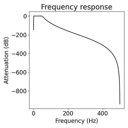
Next, we can calculate the frequency response, \(b_k\), for our IIR filter.

# Compute the frequency response for the IIR filter
f_db, db = compute_frequency_response(sos, None, fs)

# Plot the frequency response
plot_frequency_response(f_db, db)

/Users/tom/opt/anaconda3/envs/mne/lib/python3.8/site-packages/neurodsp/filt/utils.py:90: RuntimeWarning: divide by zero encountered in log10
  db = 20 * np.log10(abs(h_vals))

Above, we can see our frequency response of our filter, which shows us how different frequencies are affected by our filter. Ideally, we want zero attenuation in our passband, and a lot of attenuation in the stopband(s).

Another way to quantify these properties is the transition band, which is bandwidth (in Hz) that it takes for the filter to change from high to low attenuation. This quantifies how sharp the transition is between stopband and passband. By default, transition bands are computed as the range between -20 dB and -3 dB attenuation, but you can also customize these values.

# Compute the transition band of the filter
t_band = compute_transition_band(f_db, db)

# Print the transition band
print('Transition band: {:4.2f}'.format(t_band))

Transition band: 10.00

In the above, we have designed and evaluated an IIR filter. Note that the properties of the filter will depend on the passband and cutoff frequencies, and especially the filter order.

You can explore changing these settings to see how they impact the filter properties.

Apply

The filter we previously designed may now be applied to a signal, which can be done with the apply_iir_filter() function.

# Apply the filter to our signal
sig_filt = apply_iir_filter(sig, sos)

# Plot the filtered and original time series
plot_time_series(times, [sig, sig_filt], ['Raw', 'Filtered'])

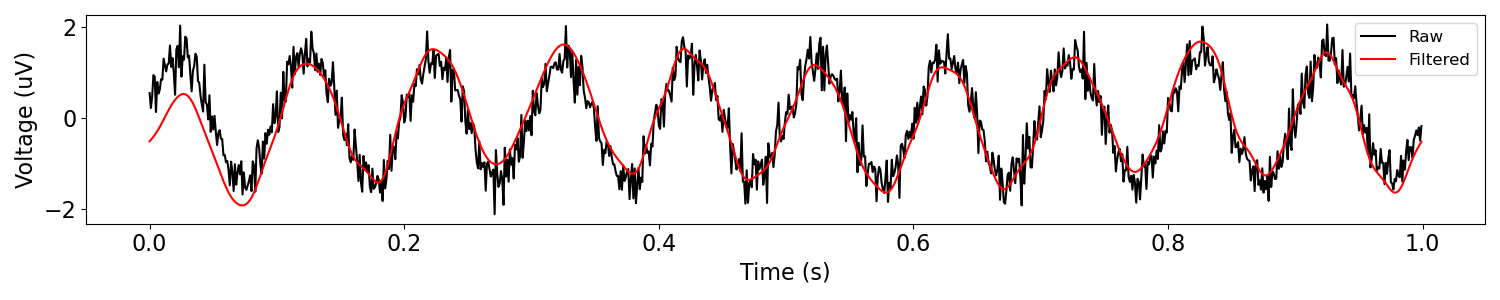
In the above, we can see both the original signal, and the filtered version.

Note that inspecting the filtered signal together with the original signal is recommended.

Using filter_signal

In the above, we did a step-by-step procedure of designing, evaluating, and applying our filter.

Note that all of these elements can also be done directly through the filter_signal() function.

sig_filt, sos = filter_signal(sig, fs, pass_type, f_range,
                              filter_type='iir', butterworth_order=butterworth_order,
                              plot_properties=True, print_transitions=True,
                              return_filter=True)

/Users/tom/opt/anaconda3/envs/mne/lib/python3.8/site-packages/neurodsp/filt/filter.py:98: UserWarning: Edge artifacts are not removed when using an IIR filter.
  warn('Edge artifacts are not removed when using an IIR filter.')
/Users/tom/opt/anaconda3/envs/mne/lib/python3.8/site-packages/neurodsp/filt/utils.py:90: RuntimeWarning: divide by zero encountered in log10
  db = 20 * np.log10(abs(h_vals))
Transition bandwidth is 10.0 Hz.
Pass/stop bandwidth is 49.0 Hz.

Example Application: Line Noise Removal

A common application of IIR filters is for line noise removal.

In this example, a 3rd order Butterworth filter is applied to remove 60Hz noise.

# Generate a signal, with a low frequency oscillation and 60 Hz line noise
components = {'sim_oscillation' : [{'freq' : 6}, {'freq' : 60}]}
variances = [1, 0.2]
sig = sim_combined(n_seconds, fs, components, variances)

# Filter settings
f_range = (58, 62)
order = 3

# Bandstop filter the data to remove line noise
sig_filt = filter_signal(sig, fs, 'bandstop', f_range,
                         filter_type='iir', butterworth_order=3)

/Users/tom/opt/anaconda3/envs/mne/lib/python3.8/site-packages/neurodsp/filt/filter.py:98: UserWarning: Edge artifacts are not removed when using an IIR filter.
  warn('Edge artifacts are not removed when using an IIR filter.')

# Plot filtered signal
plot_time_series(times, [sig, sig_filt], ['Raw', 'Filtered'])

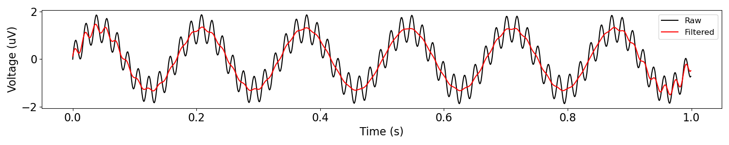
One thing you might notice in the plot above is that there are edge artifacts. The data points at the edge of the signal don’t appear to the fully filtered, and some of the high frequency activity remains. This is because data points at the edge of a signal do not get fully processed by the filter.

Note that, different from FIR filters, with IIR filters there is no simple way to remove these edges, since, due to the recursion of IIR filters, we can’t as easily define the extent of the edge effect. Because of this, edges are not automatically excluded, but as we can see edge effects can still be present, and may need to be considered.