Filter Checks

Strategies and approaches for proper filter design and application.

This tutorial covers available functionality and recommended approaches for checking and applying filters, including utilities available across neurodsp.filt.

from neurodsp.sim import sim_combined
from neurodsp.filt import filter_signal
from neurodsp.utils import create_times
from neurodsp.plts import plot_time_series

Filtering Best Practices

Although filtering can increase the signal-to-noise ratio (SNR), improper filter design may result can also introduce confounding distortions and artifacts.

In order to avoid these issues, filters need to be carefully designed and applied. Some guidelines for doing so in the context of electrophysiology data are covered in these articles:

• Widman et al., 2015

• de Cheveigne & Nelken, 2019

General recommendations based on these articles include to:

1. Consider and examine the frequency and impulse responses of the filter

2. Use simulated data to evaluate the practical effects of the filter

3. Manually inspect the filtered signal, and comparing to the original signal

When you design and apply filters with NeuroDSP, filter definition and properties checks are automatically applied with the check_filter_definition() and check_filter_properties() functions.

If you see warnings or errors when applying filters, it likely stems from these checks. Note that passing these checks does not automatically mean the filter is ideal, but at least some common issues may be caught through this process.

# Define general settings for simulations
fs = 500
n_seconds = 3
times = create_times(n_seconds, fs)

Filter Attenuation

Filter attenuation refers to the degree to which frequencies are attenuated by a filter.

You might sometimes see a user warning that warns about the level of attenuation. This warning is given whenever the constructed filter has a frequency response that does not hit a specified level of attenuation in the stopband. By default, the warning appears if the level of attenuation does not go below -20dB.

You can check filter properties by plotting the frequency response when you apply a filter.

In the following example, we will use an example of filtering out line noise, with different filter lengths that do and do not achieve sufficient attenuation.

# Generate a signal for this example, with an oscillation and 60 Hz line noise
components = {'sim_oscillation' : [{'freq' : 6}, {'freq' : 60}]}
variances = [1, 0.2]
sig = sim_combined(n_seconds, fs, components, variances)

# Define filter settings
f_range = (58, 62)
passtype = 'bandstop'

# Apply a short filter, one that won't achieve our desired attenuation
sig_filt_short = filter_signal(sig, fs, passtype, f_range,
                               n_seconds=0.25, plot_properties=True)

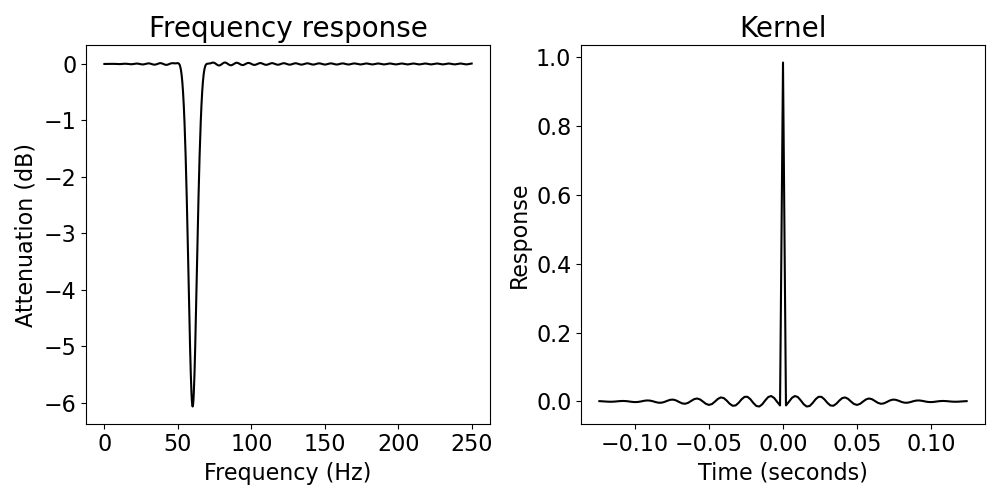
/Users/tom/opt/anaconda3/envs/mne/lib/python3.8/site-packages/neurodsp/filt/checks.py:153: UserWarning: The filter attenuation never goes below -20 dB. Increase filter length.
  warn('The filter attenuation never goes below {} dB. '\

Notice that when we apply the filter above, with a short filter length, we get a warning about the filter attenuation. The filter we have defined does not get to a sufficient attenuation level.

# This user warning disappears if we elongate the filter
sig_filt_long = filter_signal(sig, fs, passtype, f_range,
                              n_seconds=1, plot_properties=True)

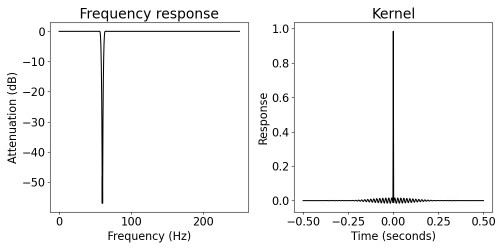
When we make the filter definition longer, we see that the warning is now gone.

To see the difference in attenuation, compare the frequency response of two filters. In particular, have a look at the scales of the frequency response, to see the different levels of attenuation each filter attains.

Time-frequency resolution trade off

When designing and applying filters, one has to keep in mind the time-frequency resolution trade off. For filters, this relates to changing the filter length. With longer filter kernels, we get improved frequency resolution, but worse time resolution. With shorter filter kernels, temporal resolution increases, but the frequency resolution is worse.

Two bandpass filters (one long and one short)

For an example, lets consider two FIR bandpass filters, with different lengths, and how this relates to their filter properties. We will once again use and compare a short and a long filter, this time focusing on the different resolutions of the outputs.

# Generate a signal with aperiodic activity, a low frequency drift, and an oscillation
components = {'sim_powerlaw' : {'exponent' : 0},
              'sim_oscillation' : [{'freq' : 1}, {'freq' : 6}]}
variances = [0.1, 1, 1]
sig = sim_combined(n_seconds, fs, components, variances)

# Set the first second to 0
sig[:fs] = 0

# Define the frequency band of interest
passband = 'bandpass'
f_range = (4, 8)

# Filter the data
sig_filt_short = filter_signal(sig, fs, passband, f_range, n_seconds=.1)
sig_filt_long = filter_signal(sig, fs, passband, f_range, n_seconds=1)

/Users/tom/opt/anaconda3/envs/mne/lib/python3.8/site-packages/neurodsp/filt/checks.py:162: UserWarning: The low or high frequency stopband never gets attenuated by more than 20 dB. Increase filter length.
  warn('The low or high frequency stopband never gets attenuated by '\
/Users/tom/opt/anaconda3/envs/mne/lib/python3.8/site-packages/neurodsp/filt/checks.py:172: UserWarning: Transition bandwidth is 10.2 Hz. This is greater than the desired pass/stop bandwidth of 4.0 Hz
  warn('Transition bandwidth is {:.1f} Hz. This is greater than the desired '\

# Plot filtered signal
plot_time_series(times, [sig, sig_filt_short, sig_filt_long],
                 ['Raw', 'Short Filter', 'Long Filter'])

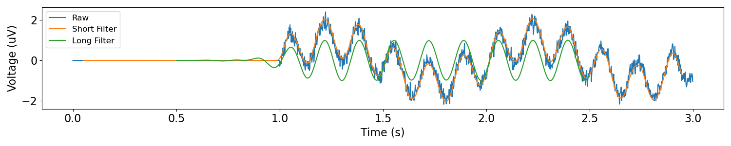
In the plot above, we can see that the short filter preserves the start of the oscillation better than the long filter (i.e. the short filter has better temporal resolution).

Notice also that the long filter correctly removed the 1Hz oscillation, but the short filter did not (i.e. the long filter has better frequency resolution).

Another way to examine these properties is by looking at the properties of the two filters.

# Filter and visualize properties for the short filter
sig_filt_short = filter_signal(sig, fs, 'bandpass', f_range, n_seconds=.1,
                               plot_properties=True)

/Users/tom/opt/anaconda3/envs/mne/lib/python3.8/site-packages/neurodsp/filt/checks.py:162: UserWarning: The low or high frequency stopband never gets attenuated by more than 20 dB. Increase filter length.
  warn('The low or high frequency stopband never gets attenuated by '\
/Users/tom/opt/anaconda3/envs/mne/lib/python3.8/site-packages/neurodsp/filt/checks.py:172: UserWarning: Transition bandwidth is 10.2 Hz. This is greater than the desired pass/stop bandwidth of 4.0 Hz
  warn('Transition bandwidth is {:.1f} Hz. This is greater than the desired '\

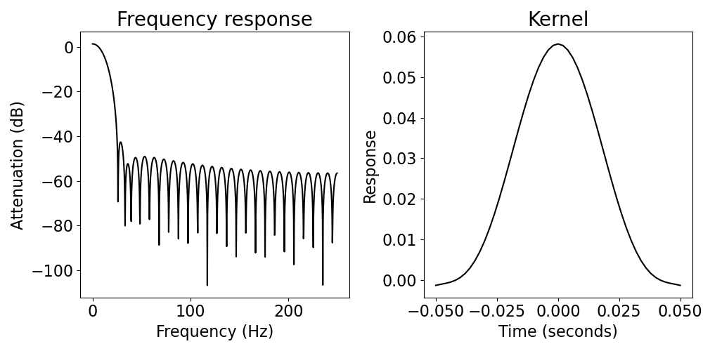
# Filter and visualize properties for the long filter
sig_filt_long = filter_signal(sig, fs, 'bandpass', f_range, n_seconds=1,
                              plot_properties=True)

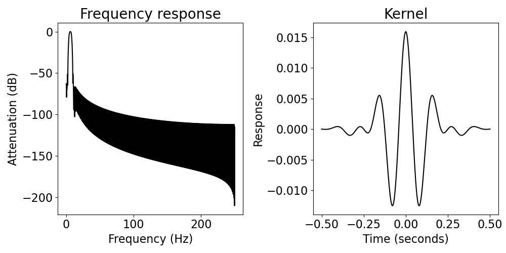
By comparing between the filter definitions for the two filters (short and long), we can see the different resolutions. Note how the short filter have a much less specific frequency response, but a much more localized impulse response. By comparison, the longer filter has a much more localized frequency response, but a more temporally diffuse impulse response.

Temporal and frequency resolution are always a trade-off, and there is no single solution to the overall “best” filter. Rather, filter design depends on the application, and whether temporal or frequency resolution is more important for a given application.

Reporting on Filters

Designing and applying appropriate filters takes some care and attention. If you are reporting on work that includes using filters, then these reports should also include information for readers to be able to assess the filters that were applied.

Following Widman et al., 2015 information that is recommended to report when using filters includes:

• Filter passtype

• Cutoff frequency and definition

• Filter order

• Transition bandwidth

• Passband ripple and stopband attenuation

• Filter delay and causality

• Direction of application