Sliding Window Matching

Find recurring patterns in neural signals using Sliding Window Matching.

This tutorial primarily covers the sliding_window_matching() function.

Overview

Non-periodic or non-sinusoidal properties can be difficult to assess in frequency domain methods. To try and address this, the sliding window matching (SWM) algorithm has been proposed for detecting and measuring recurring, but unknown, patterns in time series data. Patterns of interest may be transient events, and/or the waveform shape of neural oscillations.

In this example, we will explore applying the SWM algorithm to some LFP data.

The SWM approach tries to find recurring patterns (or motifs) in the data, using sliding windows. An iterative process samples window randomly, and compares each to the average window. The goal is to find a selection of windows that look maximally like the average window, at which point the occurrences of the window have been detected, and the average window pattern can be examined.

The sliding window matching algorithm is described in Gips et al, 2017

import numpy as np

# Import the sliding window matching function
from neurodsp.rhythm import sliding_window_matching

# Import utilities for loading and plotting data
from neurodsp.utils.download import load_ndsp_data
from neurodsp.plts.rhythm import plot_swm_pattern
from neurodsp.plts.time_series import plot_time_series
from neurodsp.utils import set_random_seed, create_times
from neurodsp.utils.norm import normalize_sig

# Set random seed, for reproducibility
set_random_seed(0)

Load neural signal

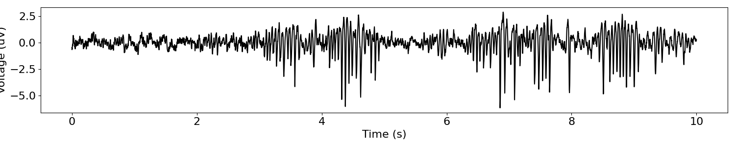
First, we will load a segment of ECoG data, as an example time series.

# Download, if needed, and load example data files
sig = load_ndsp_data('sample_data_1.npy', folder='data')
sig = normalize_sig(sig, mean=0, variance=1)

# Set sampling rate, and create a times vector for plotting
fs = 1000
times = create_times(len(sig)/fs, fs)

Next, we can visualize this data segment. As we can see this segment of data has some prominent bursts of oscillations, in this case, in the beta frequency.

# Plot example signal
plot_time_series(times, sig)

Apply sliding window matching

The beta oscillation in our data segment looks like it might have some non-sinusoidal properties. We can investigate this with sliding window matching.

Sliding window matching can be applied with the sliding_window_matching() function.

Data Preprocessing

Typically, the input signal does not have to be filtered into a band of interest to use SWM.

If the goal is to characterize non-sinusoidal rhythms, you typically won’t want to apply a filter that will smooth out the features of interest.

However, if the goal is to characterize higher frequency activity, it can be useful to apply a highpass filter, so that the method does not converge on a lower frequency motif.

In our case, the beta rhythm of interest is the most prominent, low frequency, feature of the data, so we won’t apply a filter.

Algorithm Settings

The SWM algorithm has some algorithm specific settings that need to be applied, including:

• win_len : the length of the window, defined in seconds

• win_spacing : the minimum distance between windows, also defined in seconds

The length of the window influences the patterns that are extracted from the data. Typically, you want to set the window length to match the expected timescale of the patterns under study.

For our purposes, we will define the window length to be about 1 cycle of a beta oscillation, which should help the algorithm to find the waveform shape of the neural oscillation.

# Define window length & minimum window spacing, both in seconds
win_len = .055
win_spacing = .055

# Apply the sliding window matching algorithm to the time series
windows, window_starts = sliding_window_matching(sig, fs, win_len, win_spacing, var_thresh=.5)

Examine the Results

What we got back from the SWM function are the calculate average window, the list of indices in the data of the windows, and the calculated costs for each iteration of the algorithm run.

In order to visualize the resulting pattern, we can use plot_swm_pattern().

# Compute the average window
avg_window = np.mean(windows, 0)

# Plot the discovered pattern
plot_swm_pattern(avg_window)

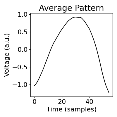
In the above average pattern, that looks to capture a beta rhythm, we can notice some waveform shape of the extracted rhythm.

Concluding Notes

One thing to keep in mind is that the SWM algorithm includes a random element of sampling and comparing the windows - meaning it is not deterministic. Because of this, results can change with different random seeds.

To explore this, go back and change the random seed, and see how the output changes.

You can also set the number of iterations that the algorithm sweeps through. Increasing the number of iterations, and using longer data segments, can help improve the robustness of the algorithm results.