Fluctuation analyses

Apply fluctuation analyses, such as detrended fluctuation analysis (DFA) to neural signals.

DFA was first proposed in the context of genetics in Peng et al, 1994, and was recently reviewed in the context of neural data in Hardstone et al, 2012.

This tutorial covers neurodsp.aperiodic.dfa.

import matplotlib.pyplot as plt

from neurodsp.sim import sim_powerlaw

# Import the function for computing fluctuation analyses
from neurodsp.aperiodic import compute_fluctuations

Detrended Fluctuation Analysis

Detrended fluctuation analysis (DFA) is a method for analyzing the self-similarity of a signal.

DFA is in some ways similar to autocorrelation measures, and is typically used to look for long-range, powerlaw correlations. It does so by dividing the signals into windows, fitting local trends, and then examining the pattern across window sizes.

For more information on the details of DFA, see the description of the algorithm on Wikipedia.

DFA Exponent

The output of the DFA algorithm is the ‘DFA exponent’, which is the slope of the linear fit between windows sizes and fluctuations. The value of this exponent can be interpreted in terms of the properties of the signal.

In particular, DFA exponents represent:

• \(0 < \alpha < 0.5\) : anti-correlated

• \(\alpha = 0.5\) : white noise

• \(0.5 < \alpha < 1\) : correlated (stationary)

• \(\alpha = 1.0\) : 1/f

• \(1 < \alpha < 2\) : correlated (non-stationary)

Applying DFA

Here, to introduce DFA, we will use colored noise signals (white noise and pink noise). These signals have different auto-correlation properties, and so should have different DFA results, which we can then compare between the signals.

Note that DFA can be applied to multiple signal types. Though here we using simulated aperiodic time series, in analyses of neural field data, DFA is most often used to examine amplitude time series of neural oscillations.

# Simulation settings
n_seconds = 10
fs = 500

# Simulate a white noise signal
sig_wn = sim_powerlaw(n_seconds, fs, exponent=0)

# Simulate a pink noise powerlaw signal
sig_pl = sim_powerlaw(n_seconds, fs, exponent=-1)

Calculating DFA

The DFA algorithm involves:

1. Removing the mean of a signal (detrending)

2. Computing the cumulative sum of the signal

3. Splitting the signal into equal-sized windows

4. Fitting a polynomial across the windows

5. Calculate the mean squared residual (fluctuation) of the fit

Steps 3-5 are repeated for various window sizes.

The DFA algorithm is available through the compute_fluctuations() function.

Algorithm Settings

The DFA algorithm requires certain settings, including:

• n_scales : the number of scales to estimate fluctuations over

• min_scale : the shortest scale, in seconds, to compute over

• max_scale : the longest scale, in seconds, to compute over

# Compute DFA for a white noise signal
ts_wn, flucs_wn, exp_wn = compute_fluctuations(sig_wn, fs, n_scales=10,
                                               min_scale=0.01, max_scale=1.0)

# Compute DFA for a pink noise signal
ts_pl, flucs_pl, exp_pl = compute_fluctuations(sig_pl, fs, n_scales=10,
                                               min_scale=0.01, max_scale=1.0)

Results

The compute_fluctuations() function returns the time scales and measured fluctuations from the DFA analysis.

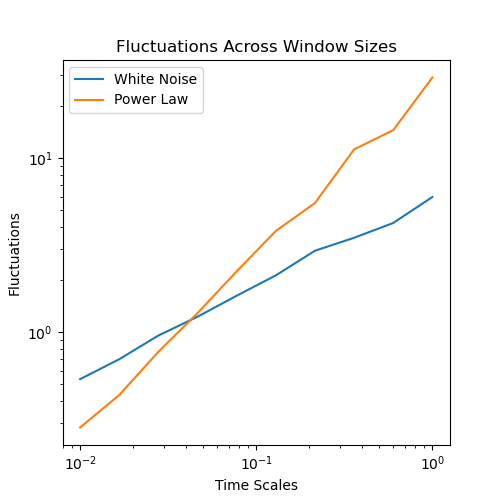
In the plot below, fluctuations are plotted across window sizes for both signals in log-log space.

_, ax = plt.subplots(figsize=(5, 5))

ax.loglog(ts_wn, flucs_wn, label="White Noise")
ax.loglog(ts_pl, flucs_pl, label="Power Law")

ax.set(title="Fluctuations Across Window Sizes",
       xlabel="Time Scales", ylabel="Fluctuations")
plt.legend();

<matplotlib.legend.Legend object at 0x7fa049043430>

The function also returns the DFA exponent, equivalent to the slope of the log-log plot of fluctuations and timescales.

# Check calculated DFA exponents
print("White noise signal DFA exponent:\t {:1.3f}".format(exp_wn))
print("Power law signal DFA exponent:\t {:1.3f}".format(exp_pl))

White noise signal DFA exponent:         0.518
Power law signal DFA exponent:   1.002

As we can see the, DFA exponent for the white noise signal is ~=0.5 while for the powerlaw signal it is ~=1. These match with the expected values for these signals.