IRASA

Separate periodic and aperiodic activity with the IRASA algorithm.

The irregular resampling auto-spectral analysis (IRASA) algorithm is a method for separating aperiodic (1/f) and oscillatory activity in the frequency domain.

The algorithm leverages the ‘scale-free’ nature of 1/f activity, resampling the data in order to separate activity with a characteristic frequency (such as periodic activity) from scale-free activity.

Briefly, this method involves:

1. Up- & down-sampling the signal across a range of increments.

2. Computing the geometric mean spectra for each pair of up/down sampled signals.

3. Estimating the aperiodic component from the median spectrum across the range of increments.

4. Estimating the periodic component from the difference between the aperiodic estimate and the original spectrum.

Full details of the IRASA algorithm are described in Wen & Liu, 2016.

This tutorial covers neurodsp.aperiodic.irasa.

import numpy as np
from neurodsp.sim import sim_combined
from neurodsp.spectral import compute_spectrum, trim_spectrum
from neurodsp.plts import plot_power_spectra

# Import IRASA related functions
from neurodsp.aperiodic import compute_irasa, fit_irasa

Simulate Data

To explore the IRASA algorithm, we’ll use a simulated signal, with a combination of aperiodic 1/f and oscillatory activity.

# Simulation settings
n_seconds = 10
fs = 500

# Define the parameters of the simulated components
cf = 10
exp = -2

# Define the components for the simulated signal
components = {'sim_oscillation' : {'freq' : cf},
              'sim_powerlaw' : {'exponent' : exp}}

# Define the frequency range of interest for the analysis
f_range = (1, 40)

# Create the simulate time series
sig = sim_combined(n_seconds, fs, components)

# Compute the power spectrum of the simulated signal
freqs, psd = compute_spectrum(sig, fs, nperseg=4*fs)

# Trim the power spectrum to the frequency range of interest
freqs, psd = trim_spectrum(freqs, psd, f_range)

# Plot the computed power spectrum
plot_power_spectra(freqs, psd, title="Original Spectrum")

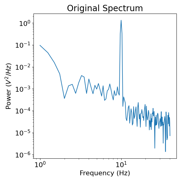
In the above spectrum, we can see a pattern of power across all frequencies, which reflects the 1/f activity, as well as a peak at 10 Hz, which represents the simulated oscillation.

IRASA

In the analysis of neural data, we may want to separate aperiodic and periodic components of the data. Here, we explore using IRASA to do so.

Algorithm Settings

The main setting for IRASA are the resampling factors to use, set by the hset input. Here, we will use default values, which are often sufficient.

In the IRASA algorithm, the periodic component is calculated as the difference between the full signal and the aperiodic component. It may be useful to apply a threshold in this calculation, to restrict the periodic component to clear ‘peaks’ above the aperiodic.

Here we will use a threshold value (thresh), such that regions of the periodic component that are not above the threshold, calculates in terms of standard deviation of the power spectrum, are left as part of the aperiodic component.

# Compute the IRASA decomposition of the data
freqs, psd_aperiodic, psd_periodic = compute_irasa(sig, fs, f_range=f_range, thresh=1)

# Plot the isolated periodic and aperiodic components
plot_power_spectra(freqs, [psd_aperiodic, psd_periodic],
                   labels=['aperiodic', 'periodic'], title="IRASA Components")

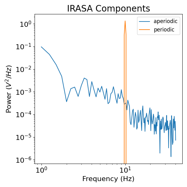
In the above components, we can see that the IRASA approach has given what appears to be a very good separation of the spectral components from our original signal.

Decomposition

Note that what IRASA returns is a decomposition of the power spectrum, separating aperiodic and periodic components.

To verify that this is what the algorithm does, we can check that the spectrum of the full signal is the same as the combined periodic and aperiodic IRASA components.

# Check that the sum of IRASA components is same as the PSD of the whole signal
psd_irasa = psd_aperiodic + psd_periodic
assert np.equal(psd_irasa, psd).all()

Subsequent Analyses

One of the goals of separating the components may be to further analyze each component.

For example, fitting the extracted aperiodic component can be done to measure the properties of the aperiodic activity. Here, we can fit the IRASA extracted aperiodic component to see if it matches what we simulated.

Note that the fitting here actually measures the slope of the power spectrum, in log-log space, which is equivalent to the 1/f exponent that was simulated.

# Fit the aperiodic component of the IRASA results
intercept, fit_sl = fit_irasa(freqs, psd_aperiodic)
print("Computed Exponent: {:1.2f}".format(fit_sl))
print("Simulated Exponent: {:1.2f}".format(exp))

Computed Exponent: -2.03
Simulated Exponent: -2.00