Note
Go to the end to download the full example code
Simulating Cycles & Transients
Simulating cycles and transient events.
This tutorial covers neurodsp.sim.cycles and neurodsp.sim.transients.
# Import utilities for simulations & plotting
from neurodsp.utils import set_random_seed
from neurodsp.plts import plot_time_series

# Import cycles
from neurodsp.sim.cycles import sim_cycle

# Import transients
from neurodsp.sim.transients import sim_damped_erp, sim_synaptic_kernel, sim_action_potential
# Set the random seed, for consistency simulating data
set_random_seed(0)

# Set some general simulation settings
fs = 1000
Simulating Cycles
NeuroDSP contains a collection of cycles that can be simulated.
The sim_cycle() function can be used to simulate individual cycles.
This function takes in a label for the type of cycle to simulate, as well as any settings for this cycle type.
Available cycles include:
sine: a sine wave cycle
asine: an asymmetric sine cycle
sawtooth: a sawtooth cycle
gaussian: a gaussian cycle
skewed_gaussian: a skewed gaussian cycle
exp: a cycle with exponential decay
2exp: a cycle with exponential rise and decay
exp_cos: an exponential cosine cycle
asym_harmonic: an asymmetric cycle made as a sum of harmonics
Note that each of these cycles also have their own function, each labeled as sim_{LABEL}_cycle.
Note that these cycles are the same as are available to simulate periodic signals.
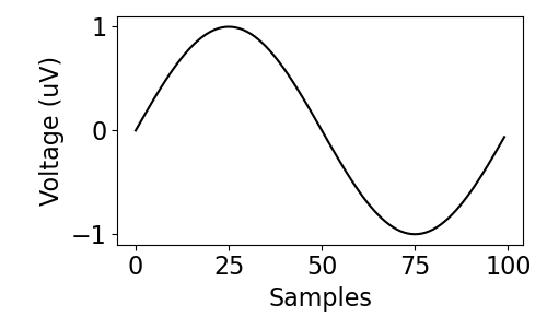
# Settings
n_seconds = 0.1

# Simulate cycle
cycle = sim_cycle(n_seconds, fs, 'sine')
# Plot simulated cycle
plot_time_series(None, cycle, figsize=(5, 3))
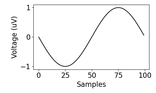
# Simulate a cycle with a phase shift
cycle = sim_cycle(n_seconds, fs, 'sine', phase=0.5)

# Plot simulated cycle
plot_time_series(None, cycle, figsize=(5, 3))
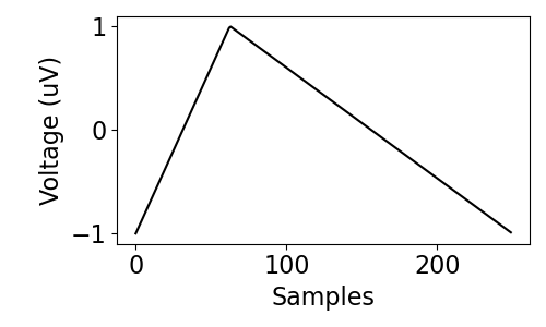
# Simulate a sawtooth cycle
cycle = sim_cycle(0.25, fs, 'sawtooth', width=0.25)

# Plot simulated cycle
plot_time_series(None, cycle, figsize=(5, 3))
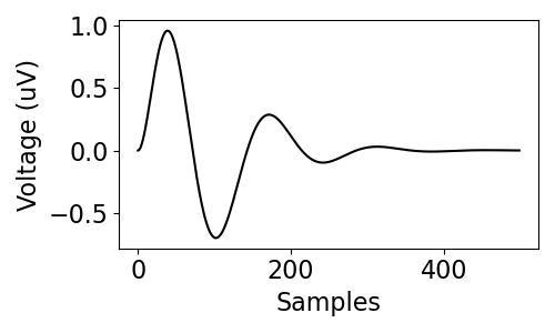
Simulating ERPs
Event-related potentials (ERPs) are transient events commonly seen in neural data.
Currently, ERPs can be simulated with the sim_dampled_erp() function,
which simulates a simplified ERP complex as an exponentially decaying sine wave.
This function takes in settings that define the amplitude and frequency of the sine wave, as well as a damping parameter.
# Reset general settings
n_seconds = 0.5

# ERP settings
amp = 1
freq = 7
decay = 0.05
# Simulate ERP
erp = sim_damped_erp(n_seconds, fs, amp, freq, decay)
# Plot the simulated ERP
plot_time_series(None, erp, figsize=(5, 3))
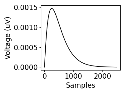
Simulate Synaptic Kernels
The sim_synaptic_kernel() function can be used to simulate synaptic kernels.
This function works by taking in rise and decay time constants.
# Reset general settings
n_seconds = 2.5

# Kernel settings
tau_r = 0.15
tau_d = 0.15
# Simulate synaptic kernel
kernel = sim_synaptic_kernel(n_seconds, fs, tau_r=0.25, tau_d=0.25)
# Plot the simulated synaptic kernel
plot_time_series(None, kernel, figsize=(4, 3))
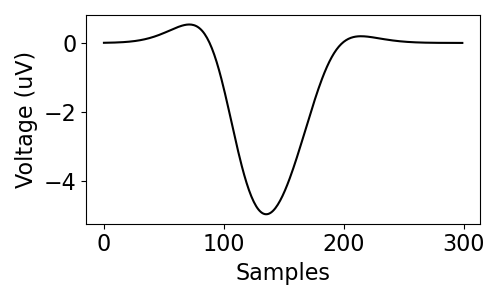
Simulating Action Potentials
There is also the sim_action_potential() function for simulating action potentials.
This function simulates an action potential as a sum of skewed Gaussians.
To create an action potential with this function, define the settings for the component skewed Gaussians.
# Reset general settings
n_seconds = 0.01
fs = 30000

# Define settings for simulating an action potential
centers = (.35, .45, .6)
stds = (.1, .1, .1)
alphas = (-1, 0, 1)
heights = (1.5, -5, 0.5)
# Simulate an action potential
ap = sim_action_potential(n_seconds, fs, centers, stds, alphas, heights)
# Plot simulated action potential
plot_time_series(None, ap, figsize=(5, 3))
Total running time of the script: ( 0 minutes 0.304 seconds)