Time-frequency analysis

Estimate instantaneous measures of phase, amplitude, and frequency.

This tutorial primarily covers the neurodsp.timefrequency module.

import matplotlib.pyplot as plt

# Import filter function
from neurodsp.filt import filter_signal

# Import time-frequency functions
from neurodsp.timefrequency import amp_by_time, freq_by_time, phase_by_time

# Import utilities for loading and plotting data
from neurodsp.utils import create_times
from neurodsp.utils.download import load_ndsp_data
from neurodsp.plts.time_series import plot_time_series, plot_instantaneous_measure

Load example neural signal

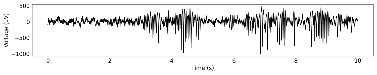
First, we will load an example neural signal to use for our time-frequency measures.

# Load a neural signal, as well as a filtered version of the same signal
sig = load_ndsp_data('sample_data_1.npy', folder='data')

# Set sampling rate, and create a times vector for plotting
fs = 1000
times = create_times(len(sig)/fs, fs)

# Set the frequency range to be used
f_range = (13, 30)

Throughout this example, we will use plot_time_series() to plot time series, and plot_instantaneous_measure() to plot instantaneous measures.

# Plot original signal
plot_time_series(times, sig)

Throughout this example, we will be examining instantaneous measures computed on the beta band.

Here, we first compute a filtered version of our signal in the beta band, which we can use for visualization purposes.

# Filter the signal into the range of interest, to use for plotting
sig_filt = filter_signal(sig, fs, 'bandpass', f_range)

# Plot filtered signal
plot_time_series(times, sig_filt)

Instantaneous Phase

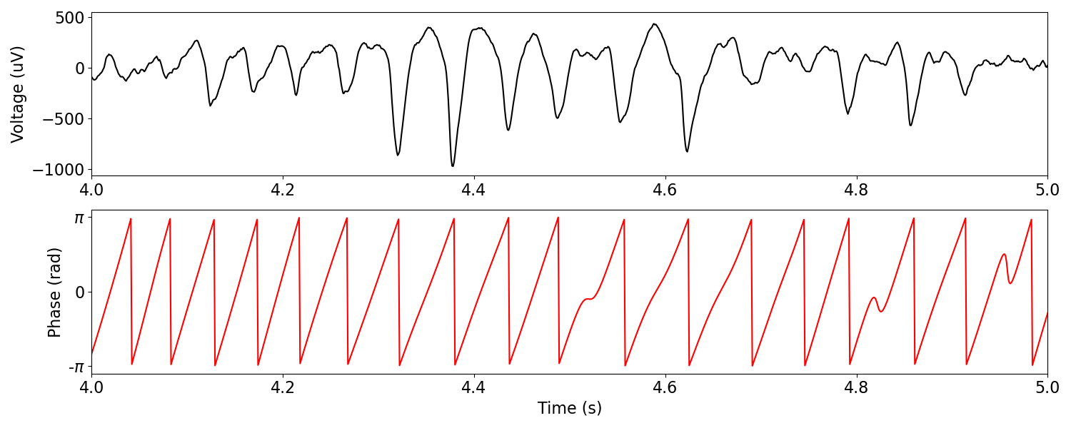
Instantaneous phase is a measure of the phase of a signal, over time.

Instantaneous phase can be analyzed with the phase_by_time() function.

Note that here we are passing in the original, unfiltered signal as well as the frequency range of interest. In doing so, the signal will be filtered prior to the instantaneous measure being computed. You can also pass in a pre-filtered signal - if so, a frequency range is not needed.

# Compute instantaneous phase from a signal
pha = phase_by_time(sig, fs, f_range)

# Plot example signal, comparing filtered trace and estimated instantaneous phase
_, axs = plt.subplots(2, 1, figsize=(15, 6))
plot_time_series(times, sig_filt, xlim=[4, 5], xlabel=None, ax=axs[0])
plot_instantaneous_measure(times, pha, colors='r', xlim=[4, 5], ax=axs[1])

Instantaneous Amplitude

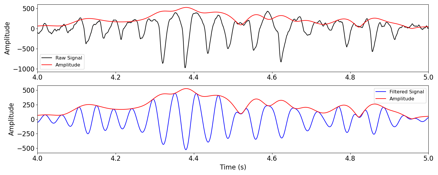
Instantaneous amplitude is a measure of the amplitude of a signal, over time.

Instantaneous amplitude can be analyzed with the amp_by_time() function.

# Compute instantaneous amplitude from a signal
amp = amp_by_time(sig, fs, f_range)

# Plot example signal
_, axs = plt.subplots(2, 1, figsize=(15, 6))
plot_instantaneous_measure(times, [sig, amp], 'amplitude',
                           labels=['Raw Signal', 'Amplitude'],
                           xlim=[4, 5], xlabel=None, ax=axs[0])
plot_instantaneous_measure(times, [sig_filt, amp], 'amplitude',
                           labels=['Filtered Signal', 'Amplitude'], colors=['b', 'r'],
                           xlim=[4, 5], ax=axs[1])

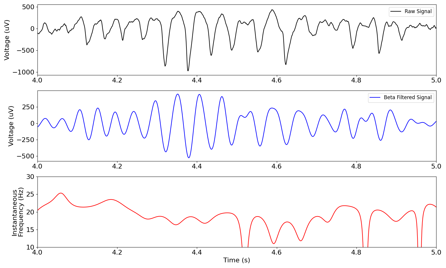
Instantaneous Frequency

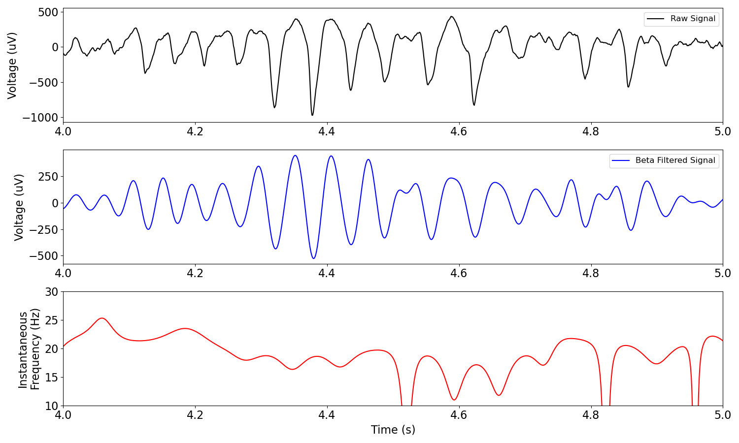
Instantaneous frequency is a measure of frequency across time.

It is measured as the temporal derivative of the instantaneous phase.

Instantaneous frequency measures can exhibit abrupt shifts. Sometimes, a transform, such as applying a median filter, is used to make it smoother.

For an example of this, see Samaha & Postle, 2015.

Instantaneous frequency can be analyzed with the freq_by_time() function.

# Compute instantaneous frequency from a signal
i_f = freq_by_time(sig, fs, f_range)

# Plot example signal
_, axs = plt.subplots(3, 1, figsize=(15, 9))
plot_time_series(times, sig, 'Raw Signal', xlim=[4, 5], xlabel=None, ax=axs[0])
plot_time_series(times, sig_filt, labels='Beta Filtered Signal',
                 colors='b', xlim=[4, 5], xlabel=None, ax=axs[1])
plot_instantaneous_measure(times, i_f, 'frequency', label='Instantaneous Frequency',
                           colors='r', xlim=[4, 5], ylim=[10, 30], ax=axs[2])