Morlet Wavelet Analysis

Perform time-frequency decomposition using wavelets.

In this tutorial we will use Morlet wavelets to compute a time-frequency representation of the data.

This tutorial primarily covers the neurodsp.timefrequency.wavelets module.

import numpy as np
from scipy import signal
import matplotlib.pyplot as plt

# Import simulation and plot code to create & visualize data
from neurodsp.sim import sim_combined
from neurodsp.plts import plot_time_series, plot_timefrequency
from neurodsp.utils import create_times

# Import function for Morlet Wavelets
from neurodsp.timefrequency.wavelets import compute_wavelet_transform

Simulate Data

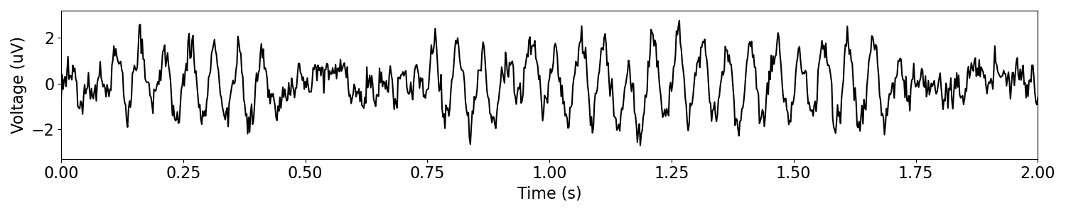
First, we’ll simulate a time series using the sim_combined() function to create a time-varying oscillation.

For this example, our oscillation frequency will be 20 Hz, with a sampling rate of 500 Hz, and a simulation time of 10 seconds.

# Define general settings for across the example
fs = 500

# Define settings for the simulated oscillation
n_seconds = 10
freq = 20
exp = -1

# Define settings for creating the simulated signal
comps = {'sim_powerlaw' : {'exponent' : exp, 'f_range' : (2, None)},
         'sim_bursty_oscillation' : {'freq' : freq}}
comp_vars = [0.25, 1]

# Simulate a signal with bursty oscillations at 20 Hz
sig = sim_combined(n_seconds, fs, comps, comp_vars)
times = create_times(n_seconds, fs)

# Plot a segment of our simulated time series
plot_time_series(times, sig, xlim=[0, 2])

Compute Wavelet Transform

Now, let’s use the compute Morlet wavelet transform algorithm to compute a time-frequency representation of our simulated data, using Morlet wavelets.

To apply the continuous Morlet wavelet transform, we need to specify frequencies of interest. The wavelet transform can then be used to compute the power at these frequencies across time.

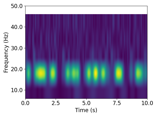
For this example, we’ll compute the Morlet wavelet transform on 50 equally-spaced frequencies from 5 Hz to 100 Hz.

# Settings for the wavelet transform algorithm
freqs = np.linspace(5, 100, 50)

# Compute wavelet transform using compute Morlet wavelet transform algorithm
mwt = compute_wavelet_transform(sig, fs=fs, n_cycles=7, freqs=freqs)

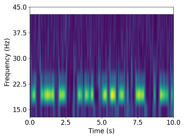
# Plot morlet wavelet transform
plot_timefrequency(times, freqs, mwt)

In the plot above, we can see the time-frequency representation from the Morlet-wavelet transformed signal.

Note that having simulated a bursty signal at 20 Hz, we can see that the time-frequency representation shows periods with high power at this frequency.

Computing wavelets across different frequency ranges

If we want to compute the time-frequency representation across a different frequency range, we can change the frequencies passed to the Morlet wavelet transform algorithm.

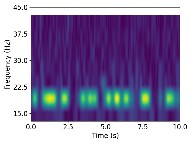
For the next example, let’s use an array of frequencies from 15 Hz to 50 Hz with a spacing of 5 Hz.

# Settings for the wavelet transform algorithm
freqs = np.arange(15, 50, 5)

# Compute wavelet transform using compute Morlet wavelet transform algorithm
mwt = compute_wavelet_transform(sig, fs=fs, n_cycles=7, freqs=freqs)

# Plot morlet wavelet transform
plot_timefrequency(times, freqs, mwt)

From the plot above, you can see the Morlet-wavelet transformed signal for the new frequency range. Again, we can see the how power at the frequency of our simulated oscillation.

Wavelet Description

Let’s look a little further into what a Wavelet is. In general, a wavelet is simply a small “wave” like signal. By sweeping this wave across our data, we can see how much of this ‘wave’ is in our signal, which is useful to quantify variations of signal amplitude across time.

A Morlet wavelet is a particular type of wavelet in which the wavelet has been multiplied by a Gaussian envelope.

Some parameters are needed to define a Morlet wavelet. These parameters are the sampling frequency, the fundamental frequency, and the number of cycles per frequency.

For more information on Morlet wavelets, see: Morlet wavelets in time and frequency a video on Youtube from Mike X Cohen.

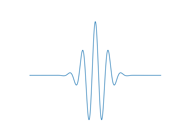
Example Plot of Morlet Wavelet

Here, we provide an example plot of an individual Morlet wavelet. We’ll use the scipy.signal function morlet to create a wavelet that is 5 cycles long.

# Define sampling rate, number of cycles, fundamental frequency, and length for the wavelet
n_cycles = 5
freq = 5
scaling = 1.0
omega = n_cycles
wavelet_len = int(n_cycles * fs / freq)

# Create wavelet
wavelet = signal.morlet(wavelet_len, omega, scaling)

# Plot the real part of the wavelet
_, ax = plt.subplots()
ax.plot(np.real(wavelet))
ax.set_axis_off()

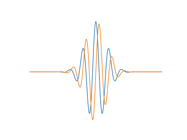
Real & Imaginary Dimensions

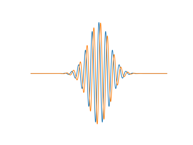
Note that wavelets have both real and imaginary dimensions.

# Plot both real and imaginary dimensions of the wavelet
_, ax = plt.subplots()
ax.plot(np.real(wavelet))
ax.plot(np.imag(wavelet))
ax.set_axis_off()

# Plot real and imaginary components in a 3D plot
fig = plt.figure()
ax = fig.add_subplot(111, projection='3d')
ax.plot(np.linspace(0, scaling, wavelet.size), wavelet.real, wavelet.imag)
ax.set(xlabel='Scaling', ylabel='Real Amplitude', zlabel='Imag Amplitude')

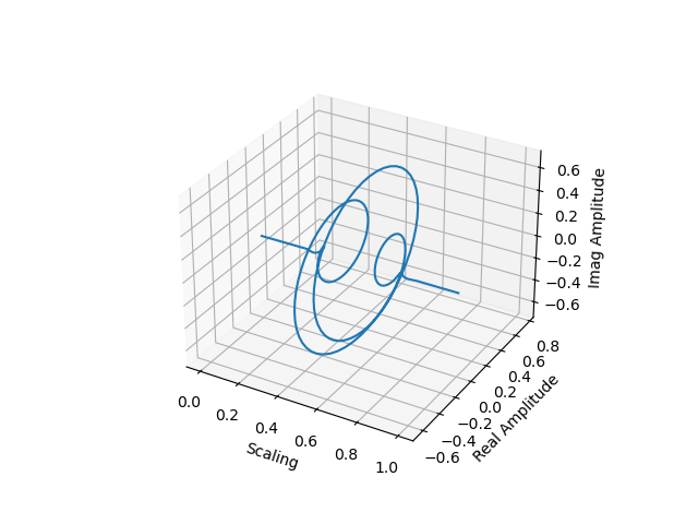
[Text(-0.04176715375665995, -0.09042854049259537, 'Scaling'), Text(0.0704766587855572, -0.07320235304988142, 'Real Amplitude'), Text(0.10787434422876363, 0.014452421710067038, 'Imag Amplitude')]

In the plots above, you can see both the real and imaginary components of the Morlet-wavelet.

Note that the function we have been using, compute_wavelet_transform() creates Morlet wavelets in the same way we have been doing here, by using the morlet function from scipy.

Changing Parameters

Adjusting the input parameters results in a different wavelet.

For example, let’s try this same plot but with a different number of cycles:

# Define settings for a new wavelet
n_cycles = 10
freq = 5
scaling = 1.0
omega = n_cycles
wavelet_len = int(n_cycles * fs / freq)

# Create wavelet
wavelet = signal.morlet(wavelet_len, omega, scaling)

# Plot wavelet
_, ax = plt.subplots()
ax.plot(np.real(wavelet))
ax.plot(np.imag(wavelet))
ax.set_axis_off()

As you can see, when you increase the n_cycles parameter, you get more oscillations (cycles) in the wavelet.

Time-Frequency Representations

Let’s now return to the Morlet wavelet transform we were originally using. How this function works is it creates wavelets, as we’ve been doing above, and then applies them to the data with the convolve_wavelet() function. This function convolves the raw signal with our complex Morlet wavelet.

The complex Morlet wavelet can be thought of as a complex sine tapered by a Gaussian. The result of the convolution returns a complex array (with real and imaginary components, like we plotted above) which represents how much power of the frequency of the wavelet was found in our signal.

Changing Parameters

Returning to the Morlet-wavelet transform algorithm, we can adjust input parameters to demonstrate how changes in the number of cycles per frequency affects the outputs.

# Compute the wavelet transform with a higher number of cycles
freqs = np.arange(15, 50, 5)
mwt = compute_wavelet_transform(sig, fs=fs, n_cycles=15, freqs=freqs)

# Plot the wavelet transform
plot_timefrequency(times, freqs, mwt)

As you can see, increasing n_cycles results in what looks like smoother pattern of activity across time. This is because the wavelets, with more cycles, are longer. This can help increase frequency resolution, but decreases temporal resolution, due to the time-frequency trade off.

If we adjust other input parameters, such as the frequency resolution, we can also get a different result.

# Compute the wavelet transform with a different set of frequencies
freqs = np.arange(10, 60, 10)
mwt = compute_wavelet_transform(sig, fs=fs, n_cycles=15, freqs=freqs)

# Plot the wavelet transform
plot_timefrequency(times, freqs, mwt)

In the above, we used a larger frequency step, with the same starting and ending frequencies.

Doing so changes the frequency resolution of our estimation.