Autocorrelation Measures

Apply autocorrelation measures to neural signals.

Autocorrelation is the correlation of a signal with delayed copies of itself. Autocorrelation measures can be useful to investigate properties of neural signals.

This tutorial covers neurodsp.aperiodic.autocorr.

import numpy as np
import matplotlib.pyplot as plt

from neurodsp.sim import sim_powerlaw, sim_oscillation

# Import the function for computing autocorrelation
from neurodsp.aperiodic import compute_autocorr

Autocorrelation Measures

Autocorrelation is computed as the correlation between the original signal and delayed copies, across different lags.

The result is a measure of how correlated a signal is to itself, across time, and the timescale of autocorrelation.

Algorithm Settings

Settings for computing autocorrelation are:

• max_lag : the maximum lag to compute autocorrelation for

• lag_step : the step size to advance across when computing autocorrelation

Both parameters are defined in samples, with defaults of using a step size of 1 sample, stepping up to a maximum lag of 1000 samples.

Autocorrelation can be computed with compute_autocorr() function, which returns timepoints at which autocorrelation was calculated, and autocorrs, which are the resulting correlation coefficients.

Autocorrelation of Periodic Signals

First, let’s examine periodic signals, specifically sine waves.

Note that periodic signals are by definition rhythmic. This means that we should expect the autocorrelation to also have a rhythmic pattern across time.

Imagine, for example, moving one sine wave across another. At some points, when they are in phase, they will line up exactly (have a high correlation), while at others, when they are out of phase, they will have either low or anti-correlation.

# Simulation settings
n_seconds = 10
fs = 1000

# Define the frequencies for the sinusoids
freq1 = 10
freq2 = 20

# Simulate sinusoids
sig_osc1 = sim_oscillation(n_seconds, fs, freq1)
sig_osc2 = sim_oscillation(n_seconds, fs, freq2)

# Compute autocorrelation on the periodic time series
timepoints_osc1, autocorrs_osc1 = compute_autocorr(sig_osc1)
timepoints_osc2, autocorrs_osc2 = compute_autocorr(sig_osc2)

Autocorrelation of a sinusoidal signal

The autocorrelation of the first sine wave is plotted below.

# Plot autocorrelations
_, ax = plt.subplots(figsize=(6, 4))
ax.plot(timepoints_osc1, autocorrs_osc1)
ax.set(xlabel='lag (samples)', ylabel='autocorrelation');

[Text(0.5, 14.722222222222216, 'lag (samples)'), Text(17.097222222222214, 0.5, 'autocorrelation')]

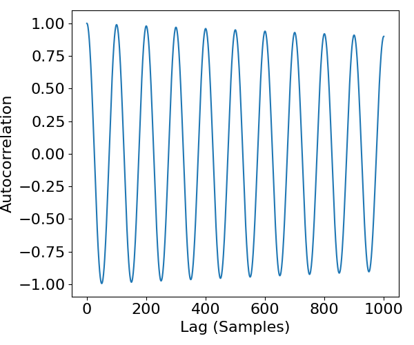
As we can see, the autocorrelation of a sinusoid is itself a sinusoid!

This reflects that a sinusoid related to itself will oscillate between being positively and negatively correlated with itself.

Next, let’s compare the autocorrelation of different sinusoids.

# Plot autocorrelations for two different sinusoids
_, ax = plt.subplots(figsize=(6, 4))
ax.plot(timepoints_osc1, autocorrs_osc1, alpha=0.75, label='10 Hz')
ax.plot(timepoints_osc2, autocorrs_osc2, alpha=0.75, label='20 Hz')
ax.set(xlabel='lag (samples)', ylabel='autocorrelation')
plt.legend(loc='upper right')

<matplotlib.legend.Legend object at 0x7fa049358e80>

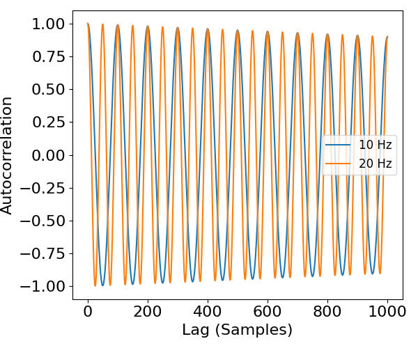
In the above, we can see that the autocorrelation of sinusoids with different frequencies leads to autocorrelation results with different timescales.

If you compare to the number of samples on the x-axis, keeping in mind the sampling rate (1000 Hz), you can check that the autocorrelation of a sinusoidal signal is a sinusoid of the same frequency.

Autocorrelation of Aperiodic Signals

Next, lets consider the autocorrelation of aperiodic signals.

Here we will use white noise, as an example of a signal without autocorrelation, and pink noise, which does, by definition, have temporal auto-correlations.

# Simulate a white noise signal
sig_wn = sim_powerlaw(n_seconds, fs, exponent=0)

# Simulate a pink noise signal
sig_pn = sim_powerlaw(n_seconds, fs, exponent=-1)

# Compute autocorrelation on the aperiodic time series
timepoints_wn, autocorrs_wn = compute_autocorr(sig_wn)
timepoints_pn, autocorrs_pn = compute_autocorr(sig_pn)

# Plot the autocorrelations of the aperiodic signals
_, ax = plt.subplots(figsize=(5, 4))
ax.plot(timepoints_wn, autocorrs_wn, label='White Noise')
ax.plot(timepoints_pn, autocorrs_pn, label='Pink Noise')
ax.set(xlabel="lag (samples)", ylabel="autocorrelation")
plt.legend()

<matplotlib.legend.Legend object at 0x7fa048eb0a60>

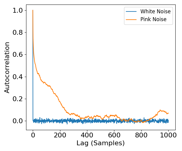
In the above, we can see that for white noise, the autocorrelation is only high at a lag of 0 samples, with all other lags being uncorrelated.

By comparison, the pink noise signal has a pattern of decreasing autocorrelation across increasing lags. This is characteristic of powerlaw data.