Simulating Combined Signals

Simulate combined signals, with periodic and aperiodic components.

This tutorial covers the neurodsp.sim.combined module.

# Import sim functions
from neurodsp.sim.combined import sim_combined, sim_peak_oscillation
from neurodsp.sim.aperiodic import sim_powerlaw
from neurodsp.utils import set_random_seed

# Import function to compute power spectra
from neurodsp.spectral import compute_spectrum

# Import utilities for plotting data
from neurodsp.utils import create_times
from neurodsp.plts.spectral import plot_power_spectra
from neurodsp.plts.time_series import plot_time_series

# Set the random seed, for consistency simulating data
set_random_seed(0)

# Set some general settings, to be used across all simulations
fs = 1000
n_seconds = 3
times = create_times(n_seconds, fs)

Simulate Combined Periodic & Aperiodic Signals

In order to simulate a signal that looks more like a brain signal, you may want to simulate an oscillation together with aperiodic activity.

We can do this with the sim_combined() function, in which you specify a set of components that you want to add together to create a complex signal.

You can use sim_combined() with any combination of any of the other simulation functions.

Each component is indicated as a string label, indicating the desired function to use, in a dictionary, with an associated dictionary of any and all parameters to use for that component as a dictionary.

# Define the components of the combined signal to simulate
components = {'sim_synaptic_current' : {'n_neurons' : 1000, 'firing_rate' : 2, 't_ker' : 1.0,
                                        'tau_r' : 0.002, 'tau_d' : 0.02},
              'sim_oscillation' : {'freq' : 8}}

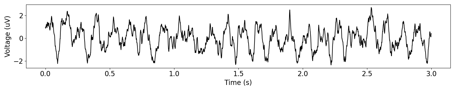
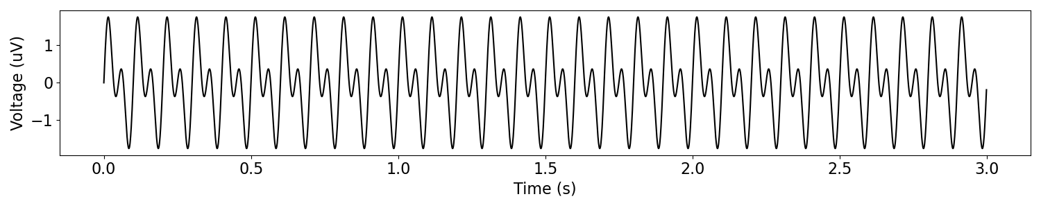
# Simulate an oscillation over an aperiodic component
signal = sim_combined(n_seconds, fs, components)

# Plot the simulated data, in the time domain
plot_time_series(times, signal)

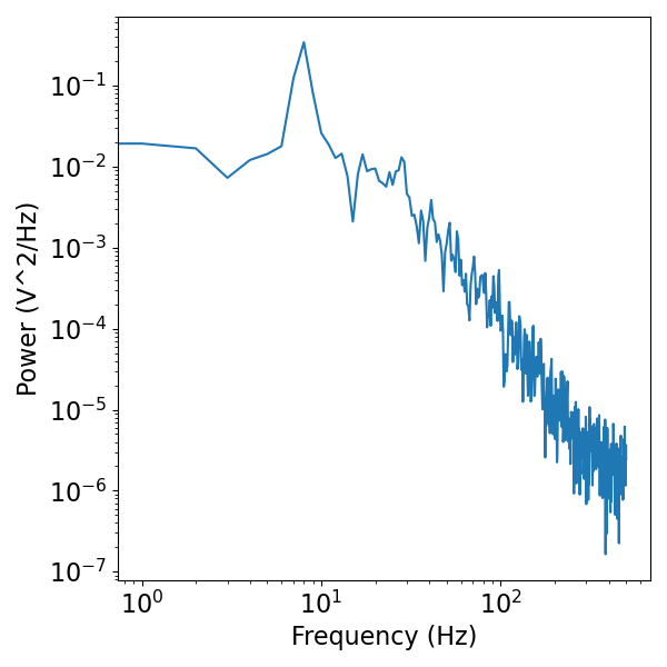
# Plot the simulated data, in the frequency domain
freqs, psd = compute_spectrum(signal, fs)
plot_power_spectra(freqs, psd)

We can switch out any components that we want, for example trading the stationary oscillation for a bursting oscillation, also with an aperiodic component.

We can also control the relative proportions of each component, by using a parameter called component_variances that specifies the variance of each component.

# Define the components of the combined signal to simulate
components = {'sim_synaptic_current' : {'n_neurons' : 1000, 'firing_rate' : 2,
                                        't_ker' : 1.0, 'tau_r' : 0.002, 'tau_d' : 0.02},
              'sim_bursty_oscillation' : {'freq' : 10}}
component_variances = [1, 0.5]

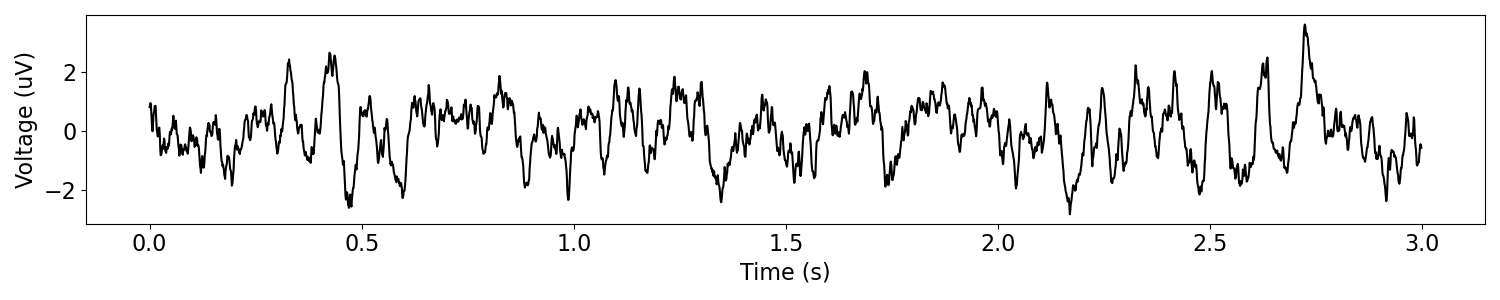
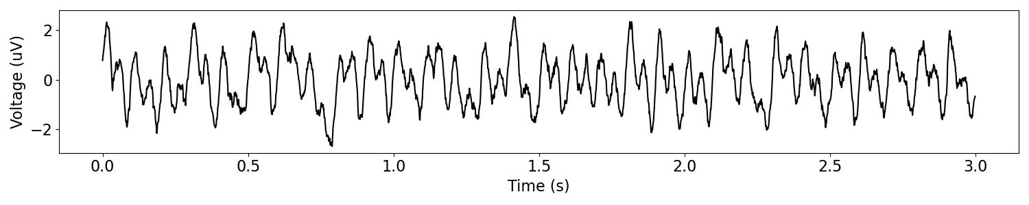
# Simulate a bursty oscillation combined with aperiodic activity
sig = sim_combined(n_seconds, fs, components, component_variances)

# Plot the simulated data, in the time domain
plot_time_series(times, sig)

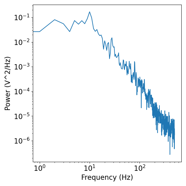
# Plot the simulated data, in the frequency domain
freqs, psd = compute_spectrum(sig, fs)
plot_power_spectra(freqs, psd)

Simulating Multiple Components from the Same Function

If you wish, you can also combine multiple components from the same simulation function.

To do so, replace the dictionary of parameters with a list of parameters, where each entry is a dictionary for each component, using the same simulation function.

# Define the components of a signal with multiple oscillatory components
components = {'sim_oscillation' : [{'freq' : 10}, {'freq' : 20}]}

# Simulate a combined signal with multiple oscillations
sig = sim_combined(n_seconds, fs, components)

# Plot the simulated data, in the time domain
plot_time_series(times, sig)

This can also be combined with other types of components.

For example, here we can combine multiple oscillations with an aperiodic component, while also controlling the relative proportions of each.

# Define the components of the combined signal to simulate
components = {'sim_powerlaw' : {'exponent': -2, 'f_range' : [2, None]},
              'sim_oscillation' : [{'freq' : 10}, {'freq' : 20}]}
component_variances = [0.5, 1, 1]

# Simulate a combined signal with multiple oscillations
sig = sim_combined(n_seconds, fs, components)

# Plot the simulated data, in the time domain
plot_time_series(times, sig)

Simulate Peak Oscillation

Next, we will simulate a time series with a peak in the power spectrum, that we can define in terms of the specific location and shape of the oscillatory peak.

In order to make this simulation, we precompute an aperiodic signal, to which we can add an oscillatory component to make the overall signal.

To do so, we use the sim_peak_oscillation() function to add an oscillation to the aperiodic component, specifying a desired central frequency, bandwidth, and peak height.

# Precompute an aperiodic time series
ap_sig = sim_powerlaw(n_seconds, fs, exponent=-1)

# Define settings that define the peak to add
freq = 10
bw = 3
height = 2

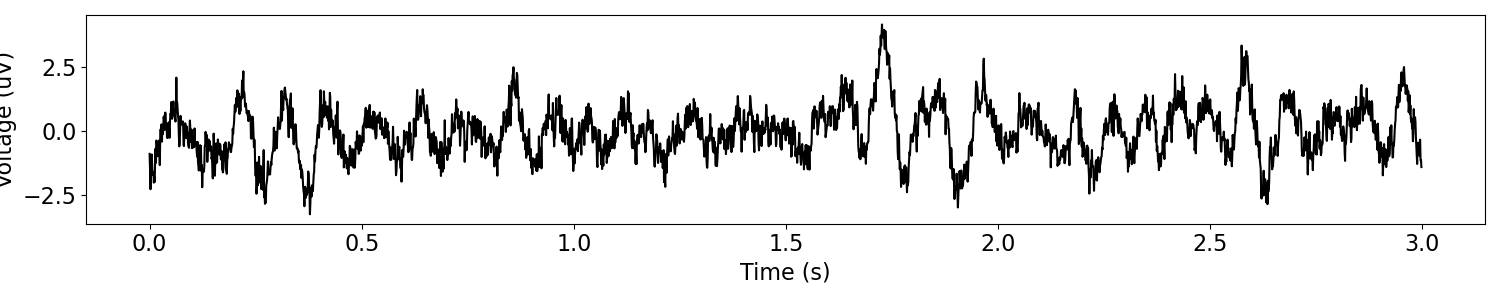
# Simulate the peak oscillation signal
sig = sim_peak_oscillation(ap_sig, fs, freq, bw, height)

# Plot the simulated data, in the time domain
plot_time_series(times, sig)

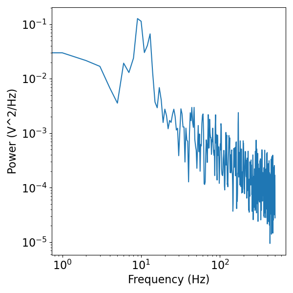
# Plot the simulated data, in the frequency domain
freqs, psd = compute_spectrum(sig, fs)
plot_power_spectra(freqs, psd)