Simulating Periodic Signals

Simulate periodic, or oscillatory, signals.

This tutorial covers the neurodsp.sim.periodic module.

import numpy as np

# Import sim functions
from neurodsp.sim import (sim_oscillation, sim_bursty_oscillation,
                          sim_variable_oscillation, sim_damped_oscillation)
from neurodsp.utils import set_random_seed

# Import function to compute power spectra
from neurodsp.spectral import compute_spectrum

# Import utilities for plotting data
from neurodsp.utils import create_times
from neurodsp.plts.spectral import plot_power_spectra
from neurodsp.plts.time_series import plot_time_series

# Set the random seed, for consistency simulating data
set_random_seed(0)

# Set some general settings, to be used across all simulations
fs = 1000

Simulate a Stationary Oscillation

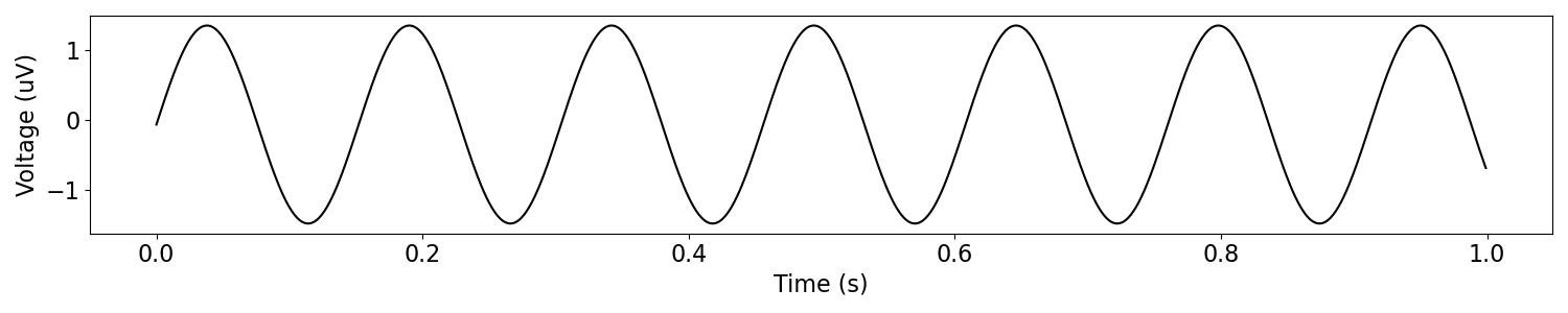
Let’s start by simulating an oscillation. We’ll start with a simple, sinusoidal, oscillation.

Continuous periodic signals can be created with sim_oscillation().

# Simulation settings
n_seconds = 1
times = create_times(n_seconds, fs)

# Define oscillation frequency
osc_freq = 6.6

# Simulate a sinusoidal oscillation
osc_sine = sim_oscillation(n_seconds, fs, osc_freq, cycle='sine')

# Plot the simulated data, in the time domain
plot_time_series(times, osc_sine)

Cycle Kernels

To simulate oscillations, we can use a sinusoidal kernel, as above, or any of a selection of other cycle kernels.

Different kernels represent different shapes and properties that may be useful to simulate different aspects of periodic neural activity.

Cycle kernel options include:

• sine: a sine wave cycle

• asine: an asymmetric sine wave

• sawtooth: a sawtooth wave

• gaussian: a gaussian cycle

• skewed_gaussian : a skewed gaussian cycle

• exp: a cycle with exponential decay

• 2exp: a cycle with exponential rise and decay

• exp_cos: an exponential cosine cycle

• asym_harmonic: an asymmetric cycle made as a sum of sinusoids

Note that these cycle kernels are all created with the sim_cycle() function.

Simulate a Shapely Oscillation

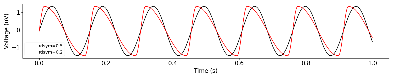
Next let’s simulate an asymmetric oscillation, using the asine cycle kernel, which stands for ‘asymmetric sinusoidal’.

Using the asine kernel, we can simulate arbitrary rise-decay symmetry of oscillations.

We’ll plot it over our original sinusoidal oscillation, so we can compare them.

# Define settings
rdsym = 0.2

# Simulate a non-sinusoidal oscillation
osc_shape = sim_oscillation(n_seconds, fs, osc_freq,
                            cycle='asine', rdsym=rdsym)

# Plot the simulated data, in the time domain
plot_time_series(times, [osc_sine, osc_shape],
                 labels=['rdsym='+str(.5), 'rdsym='+str(rdsym)])

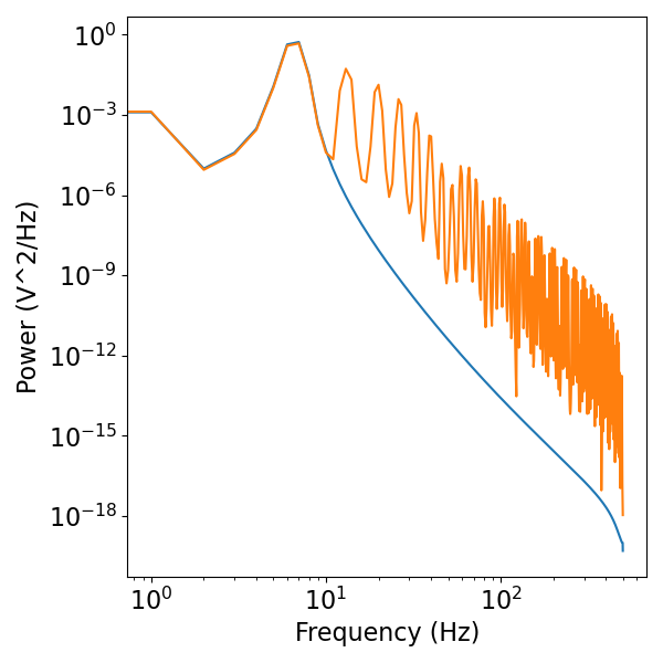
We can also compare these signals in the frequency domain.

Notice that the asymmetric oscillation has strong harmonics resulting from the non-sinusoidal nature of the oscillation.

# Plot the simulated data, in the frequency domain
freqs_sine, psd_sine = compute_spectrum(osc_sine, fs)
freqs_shape, psd_shape = compute_spectrum(osc_shape, fs)

plot_power_spectra([freqs_sine, freqs_shape], [psd_sine, psd_shape])

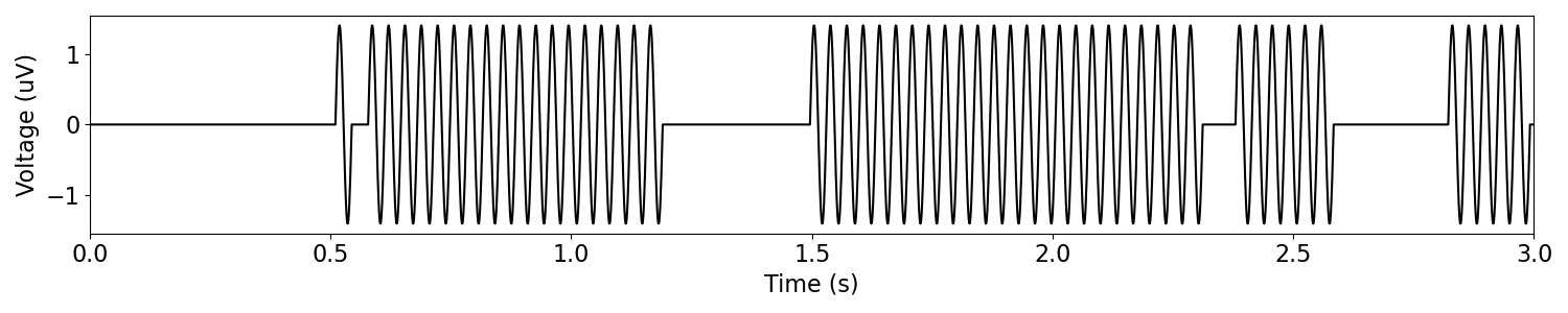
Simulate a Bursty Oscillation

Sometimes we want to study oscillations that come and go, so it can be useful to simulate oscillations with this property.

Bursty oscillations can be simulated with sim_bursty_oscillation().

Burst Probability

One way to control the bursty-ness of the simulated signal, is to control the probability that a burst will start or stop with each new cycle.

# Simulation settings
n_seconds = 3
times = create_times(n_seconds, fs)

# Define oscillation frequency
osc_freq = 30

# Burst settings
enter_burst = 0.1
leave_burst = 0.1

# Simulate a bursty oscillation
burst = sim_bursty_oscillation(n_seconds, fs, osc_freq,
                               enter_burst=enter_burst,
                               leave_burst=leave_burst)

# Plot the simulated burst signal
plot_time_series(times, burst, xlim=[0, n_seconds])

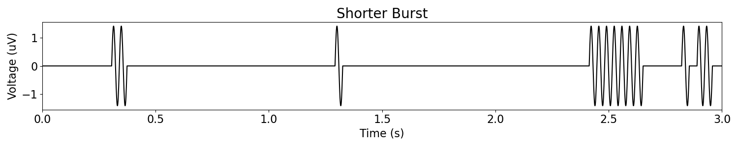
By updating the burst settings, we can change the overall probability of bursting.

For example, we can shorten burst duration by increasing the probability to leave bursts.

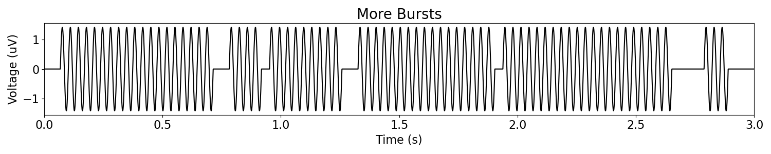
Alternatively, we can increase the number of bursts by increasing the probability to enter a burst.

# Simulate a bursty oscillation, with a higher probability to leave bursts
short_burst = sim_bursty_oscillation(n_seconds, fs, osc_freq,
                                     enter_burst=0.1, leave_burst=0.4)

# Simulate a bursty oscillation, with a higher probability of entering bursts
more_bursts = sim_bursty_oscillation(n_seconds, fs, osc_freq,
                                     enter_burst=0.4, leave_burst=0.1)

# Plot the simulated burst signals
plot_time_series(times, short_burst, xlim=[0, n_seconds], title='Shorter Burst')

plot_time_series(times, more_bursts, xlim=[0, n_seconds], title='More Bursts')

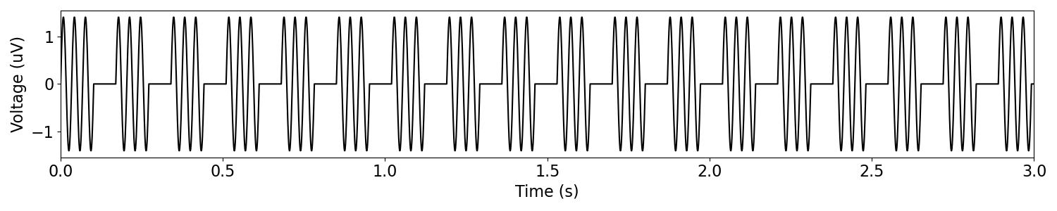
Burst Durations

Another way to control the bursty-ness is to define the burst durations.

Still using sim_bursty_oscillation(), rather than defining burst probabilities, we can define the number of cycle within / between bursts.

# Burst settings
burst_params = dict(n_cycles_burst=3, n_cycles_off=2)

# Simulate a bursty oscillation, defined in terms of durations
burst = sim_bursty_oscillation(n_seconds, fs, osc_freq, 'durations',
                               burst_params=burst_params)

# Plot the simulated burst signal
plot_time_series(times, burst, xlim=[0, n_seconds])

Simulate Variable Oscillations

Another option is to simulate oscillations that vary in their parameters over time.

To do this, we can use sim_variable_oscillation(), which allows for defining parameters per cycle.

# Define variable frequencies
freqs = np.tile([10, 12, 10, 8, 6, 8], 5)

# Simulate variable oscillatory signal
variable = sim_variable_oscillation(n_seconds, fs, freqs)

# Plot the simulated variable signal
plot_time_series(times, variable, xlim=[0, n_seconds])

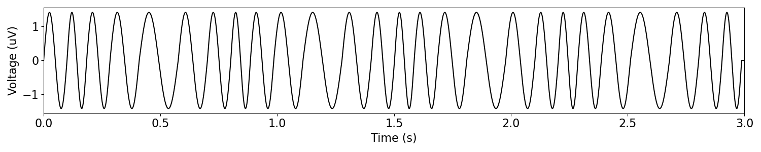
In the above, we defined a variable frequency for a sinusoidal signal.

We can also define cycle-by-cycle values for other parameters, including for other cycle types.

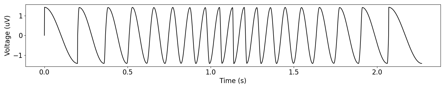
# Define ranges of frequencies and rise decay symmetries
freqs = np.concatenate([np.linspace(5, 14, 10), np.linspace(13, 5, 9)])
rdsyms = np.concatenate([np.linspace(0, .9, 10), np.linspace(.8, 0, 9)])

# Simulate variable oscillatory signal
variable = sim_variable_oscillation(None, fs, freqs, cycle='asine', rdsym=rdsyms)

# Plot the simulated variable signal
times = np.arange(0, len(variable)/fs, 1/fs)

plot_time_series(times, variable)

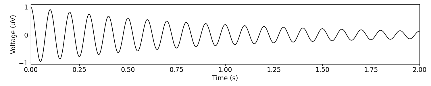
Simulate Damped Oscillations

We can also simulated damped oscillations, using sim_damped_oscillation().

# Reset general simulation settings
n_seconds = 2.
times = create_times(n_seconds, fs)

# Define oscillation frequency
osc_freq = 10

# Define dampening parameters
damping = 1.

# Simulate a damped oscillation
damped = sim_damped_oscillation(n_seconds, fs, osc_freq, damping)

# Plot the simulated damped oscillation
plot_time_series(times, damped, xlim=[0, n_seconds])