Lagged Coherence

Calculate the rhythmicity of neural signal with the lagged coherence algorithm.

This tutorial primarily covers the compute_lagged_coherence() function.

Overview

Lagged coherence is a measure to quantify the rhythmicity of neural signals.

Lagged coherence works by quantifying phase consistency between non-overlapping data fragments, calculated with Fourier coefficients. The consistency of the phase differences across epochs indexes the rhythmicity of the signal. Lagged coherence can be calculated for a particular frequency, and/or across a range of frequencies of interest.

The lagged coherence algorithm is described in Fransen et al, 2015

import numpy as np

# Import the lagged coherence function
from neurodsp.rhythm import compute_lagged_coherence

# Import functions for simulating data
from neurodsp.sim import sim_powerlaw, sim_combined
from neurodsp.utils import set_random_seed, create_times

# Import utilities for loading and plotting
from neurodsp.utils.download import load_ndsp_data
from neurodsp.plts.time_series import plot_time_series
from neurodsp.plts.rhythm import plot_lagged_coherence

# Set the random seed, for consistency simulating data
set_random_seed(0)

Simulate an Example Signal

First, let’s start by creating some simulated data, to which we can apply lagged coherence.

Simulation Settings

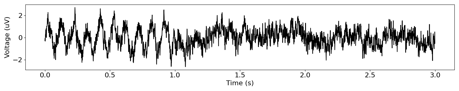
We’ll start with an example signal that starts with a burst of alpha activity, followed by a period of only aperiodic activity.

# Set the sampling rate
fs = 1000

# Set time for each segment of the simulated signal, in seconds
t_osc = 1           # oscillation
t_ap = 2            # aperiodic

# Set the frequency of the oscillation
freq = 10

# Set the exponent value for the aperiodic activity
exp = -1

# Create a times vector
times = create_times(t_osc + t_ap, fs)

Create the simulated data

Next, we will create our simulated data, by concatenating simulated segments of data with and without a rhythm.

# Simulate a signal component with an oscillation
components = {'sim_oscillation' : {'freq' : freq},
                      'sim_powerlaw' : {'exponent' : exp, 'f_range' : (1, None)}}
s1 = sim_combined(t_osc, fs, components, [1, 0.5])

# Simulate a signal component with only aperiodic activity
s2 = sim_powerlaw(t_ap, fs, exp, variance=0.5)

# Join signals together to approximate a 'burst'
sig = np.append(s1, s2)

# Plot example signal
plot_time_series(times, sig)

Compute lagged coherence on simulated data

We can compute lagged coherence with the compute_lagged_coherence() function.

Data Preprocessing & Algorithm Settings

The lagged coherence calculates the FFT across segments of the input data, and examines phase properties of frequencies of interest. As a spectral method that relies of the Fourier transform, the data does not have to be filtered prior to applying lagged coherence.

You do have to specify which frequencies to examine the lagged coherence for, which is provided to the function as the freqs input. This input, which can specify either a list or a range of frequencies, indicates which frequencies to analyze with lagged coherence.

An optional setting is the number of cycles to use at each frequency. This parameter controls the segment size used for each frequency.

# Set the frequency range to compute lagged coherence across
f_range = (8, 12)

Apply Lagged Coherence

Next, we can apply the lagged coherence algorithm to get the average lagged coherence across the alpha range.

# Compute lagged coherence
lag_coh_alpha = compute_lagged_coherence(sig, fs, f_range)

Lagged coherence result

The resulting lagged coherence value is bound between 0 and 1, with higher values indicating greater rhythmicity in the signal.

# Check the resulting value
print('Lagged coherence = ', lag_coh_alpha)

Lagged coherence =  0.6981128683467895

The calculated lagged coherence value in the alpha range is high, meaning our measured lagged coherence value is indicating a large amount of rhythmicity across the analyzed frequencies. This is expected, since our simulated signal contains an alpha oscillation.

Compute lagged coherence across the frequency spectrum

What we calculated above was the average lagged coherence across a frequency range of interest, specifically the alpha range of (8, 12).

Instead of looking at the average lagged coherence across a range, we can also calculated the lagged coherence for each frequency, and then look at the the distribution of lagged coherence values.

To do so, we can set the return_spectrum parameter to be True, to indicated the function to return the full spectrum of lagged coherence values, as opposed to the average across the given range.

# Set the frequency range to compute the spectrum of LC values across
lc_range = (5, 40)

# Calculate lagged coherence across a frequency range
lag_coh_by_f, freqs = compute_lagged_coherence(sig, fs, lc_range, return_spectrum=True)

Our outputs for lagged coherence are now a vector of lagged coherence values, as well as a vector of the frequencies that they correspond to.

To visualize this result, we can use the plot_lagged_coherence() function.

# Visualize lagged coherence as a function of frequency
plot_lagged_coherence(freqs, lag_coh_by_f)

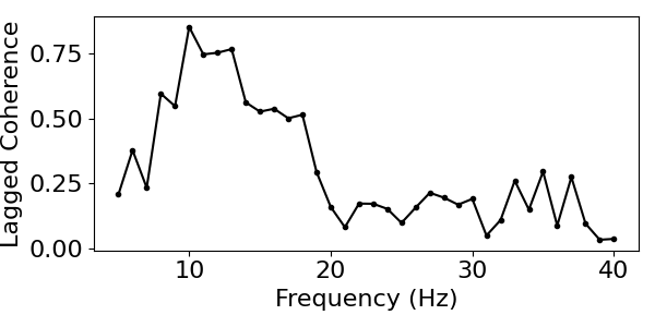
In these results, the lagged coherence peaks around 10 Hz. This is expected, as that is the frequency of the oscillation that we simulated, and the signal contains no other rhythms.

Notice, however, that the peak around 10 Hz is not very specific to that frequency (it’s quite broad). This reflects the frequency resolution of the measure.

The frequency resolution is controlled by the n_cycles parameter. You can explore how the spectrum of lagged coherence values varies as you chance the n_cycles input.

Compute lagged coherence for segments with and without bursts

Another factor we may want to keep in mind is that we are analyzing a signal with a bursty oscillation, and averaging the lagged coherence across the entire time range.

To examine how the measure varies when the oscillation is and is not present, we can restrict our analysis to particular segments of the signal.

In the following, we will apply lagged coherence separately to the bursting and non-bursting segments of the data.

# Calculate coherence for data segment with the oscillation present
lc_burst = compute_lagged_coherence(sig[0:t_osc*fs], fs, f_range)

# Calculate coherence for data segment without the alpha present burst
lc_noburst = compute_lagged_coherence(sig[t_osc*fs:2*fs*t_ap], fs, f_range)

print('Lagged coherence, bursting = ', lc_burst)
print('Lagged coherence, not bursting = ', lc_noburst)

Lagged coherence, bursting =  0.9809114285238912
Lagged coherence, not bursting =  0.357112530688723

Compute lagged coherence of an example neural signal

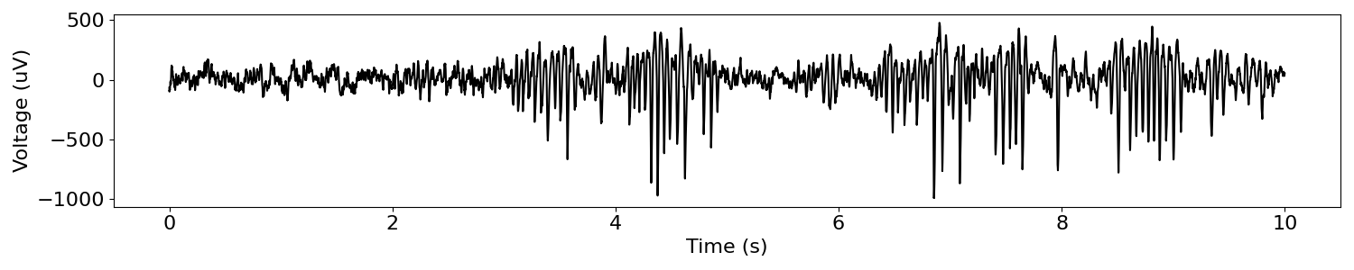
Finally, let’s apply the lagged coherence algorithm to some real data.

First we can load and plot a segment of real data, which in this case is a segment of ECoG data with a beta oscillation.

# Download, if needed, and load example data file
sig = load_ndsp_data('sample_data_1.npy', folder='data')
sig_filt_true = load_ndsp_data('sample_data_1_filt.npy', folder='data')

# Set sampling rate, and create a times vector for plotting
fs = 1000
times = create_times(len(sig)/fs, fs)

# Plot example signal
plot_time_series(times, sig)

Now let’s apply lagged coherence to the loaded data. In this data, we suspect rhythmicity in the beta range, so that is the range that we will examine with lagged coherence.

# Set the frequency range to compute lagged coherence across
beta_range = (13, 30)

# Compute lagged coherence across the beta range in the real data
lc_betas, freqs_beta = compute_lagged_coherence(sig, fs, beta_range, return_spectrum=True)

# Plot the distribution of lagged coherence values in the real data
plot_lagged_coherence(freqs_beta, lc_betas)

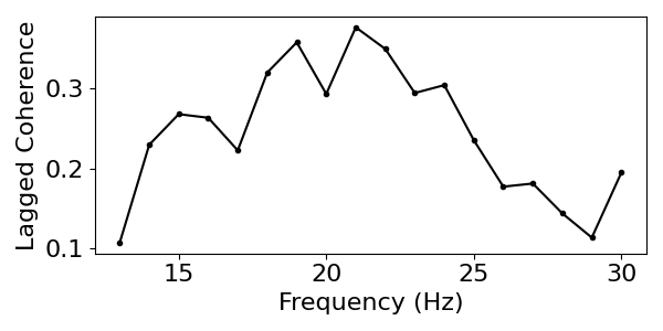
Concluding Notes

In the above, we can see a pattern of lagged coherence across the examined range, that is consistent with beta rhythmicity.

To further explore this, we might want to examine the robustness by trying different values for n_cycles, and/or comparing the this result to peaks in the power spectrum, and/or with burst detection results.