Simulating Aperiodic Signals

Simulate aperiodic signals.

This tutorial covers the the neurodsp.sim.aperiodic module.

# Import sim functions
from neurodsp.sim import (sim_powerlaw, sim_random_walk, sim_synaptic_current,
                          sim_knee, sim_frac_gaussian_noise, sim_frac_brownian_motion)
from neurodsp.utils import set_random_seed

# Import function to compute power spectra
from neurodsp.spectral import compute_spectrum

# Import utilities for plotting data
from neurodsp.utils import create_times
from neurodsp.plts.spectral import plot_power_spectra
from neurodsp.plts.time_series import plot_time_series

# Set the random seed, for consistency simulating data
set_random_seed(0)

# Set some general settings, to be used across all simulations
fs = 1000
n_seconds = 10

# Create a times vector for the simulations
times = create_times(n_seconds, fs)

Simulate 1/f Activity

Often, we want to simulate aperiodic activity similar to what we see in neural recordings.

Neural signals display 1/f-like activity, whereby power decreases linearly across increasing frequencies, when plotted in log-log.

To simulate activity with powerlaw distributions, use the sim_powerlaw() function.

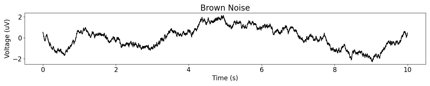
Let’s start with a power law signal, specifically a brown noise process, or a signal for which the power spectrum is distributed as 1/f^2.

# Set the exponent for brown noise, which is -2
exponent = -2

# Simulate powerlaw activity
br_noise = sim_powerlaw(n_seconds, fs, exponent)

# Plot the simulated data, in the time domain
plot_time_series(times, br_noise, title='Brown Noise')

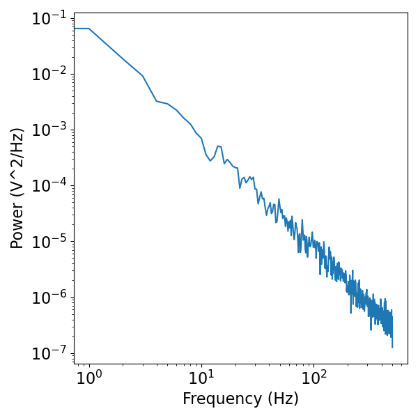
# Plot the simulated data, in the frequency domain
freqs, psd = compute_spectrum(br_noise, fs)
plot_power_spectra(freqs, psd)

Simulate Filtered 1/f Activity

The power law simulation function is also integrated with a filter. This can be useful for filtering out some low frequencies, as is often done with neural signals, to remove the very slow drifts that we see in the pure 1/f simulations.

To filter a simulated power law signal, simply pass in a filter range, and the filter will be applied to the simulated data before being returned.

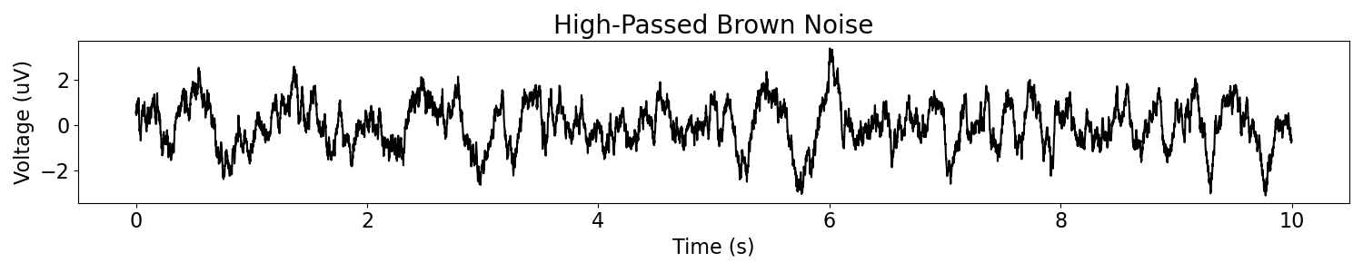
Here we will apply a high-pass filter. We can see that the resulting signal has much less low-frequency drift than the first one.

# Simulate highpass-filtered brown noise with a 1Hz highpass filter
f_hipass_brown = 1
brown_filt = sim_powerlaw(n_seconds, fs, exponent, f_range=(f_hipass_brown, None))

# Plot the simulated data, in the time domain
plot_time_series(times, brown_filt, title='High-Passed Brown Noise')

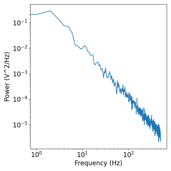
# Plot the simulated data, in the frequency domain
freqs, psd = compute_spectrum(brown_filt, fs)
plot_power_spectra(freqs, psd)

Note: the sim_powerlaw() function can simulate arbitrary power law exponents, such as pink noise (-1), or any other exponent.

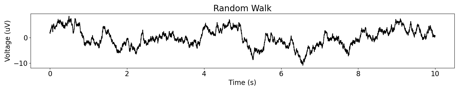
Random Walk Activity

We can also simulate an Ornstein-Uhlenbeck process, which is a random walk process with memory.

We can do this with the sim_random_walk() function.

# Simulate aperiodic signals from a random walk process
rw_ap = sim_random_walk(n_seconds, fs)

# Plot the simulated data, in the time domain
plot_time_series(times, rw_ap, title='Random Walk')

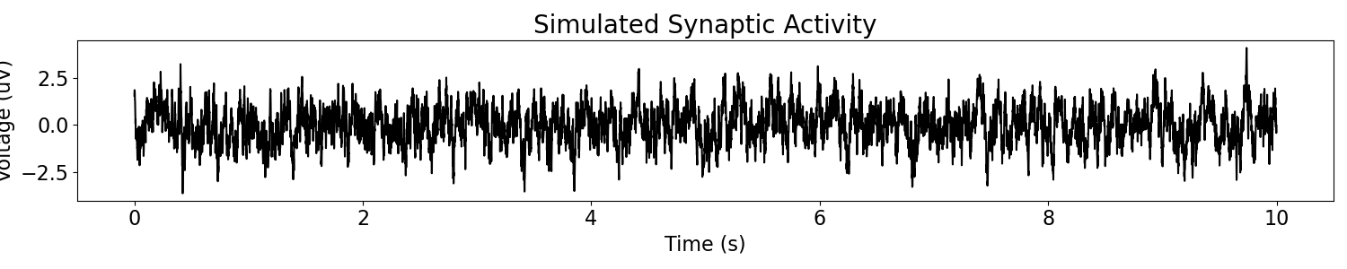
Simulate Synaptic Activity

Another model for simulating aperiodic, neurally plausible activity, is to simulate synaptic current activity, as a Lorentzian function.

This is available with the sim_synaptic_current() function.

The synaptic current model is Poisson activity convolved with exponential kernels that mimic the shape of post-synaptic potentials.

For more details on the usage of such models for simulating neural signals, see Gao et al, 2017.

# Simulate aperiodic activity from the synaptic kernel model
syn_ap = sim_synaptic_current(n_seconds, fs)

# Plot the simulated data, in the time domain
plot_time_series(times, syn_ap, title='Simulated Synaptic Activity')

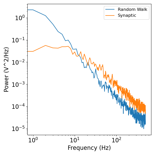
Both the random walk, and synaptic model produce 1/f scaling in higher frequencies with a fixed exponent of -2, as we can see in the power spectra plot below.

# Plot the simulated data, in the frequency domain
freqs, rw_psd = compute_spectrum(rw_ap, fs)
freqs, syn_psd = compute_spectrum(syn_ap, fs)

plot_power_spectra(freqs, [rw_psd, syn_psd], ['Random Walk', 'Synaptic'])

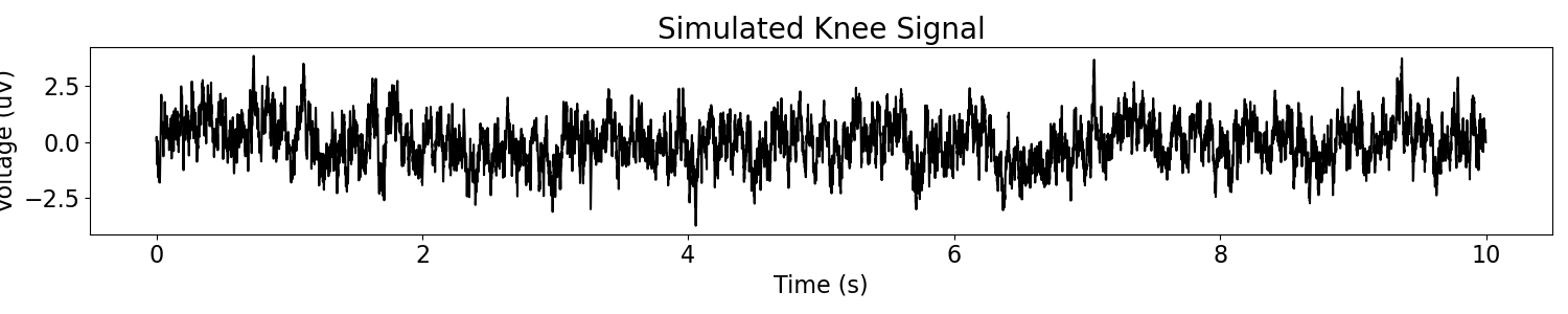
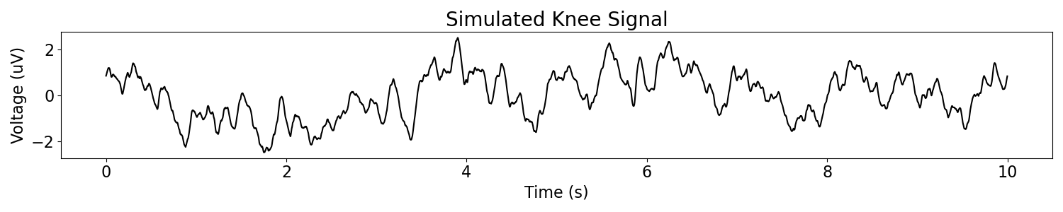
Simulate Knee Signal

To simulate signals with a knee, being able to control both exponents, and the knee, use the sim_knee() function.

# Simulate a knee signal, with specified exponents & knee
knee_ap1 = sim_knee(n_seconds, fs, exponent1=-0.5, exponent2=-1, knee=100)

# Plot the simulated data, in the time domain
plot_time_series(times, knee_ap1, title='Simulated Knee Signal')

# Simulate another knee signal, with different exponents & knee
knee_ap2 = sim_knee(n_seconds, fs, exponent1=-1, exponent2=-2, knee=100)

# Plot the simulated data, in the time domain
plot_time_series(times, knee_ap2, title='Simulated Knee Signal')

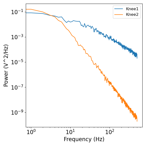
# Compute power spectra of the simulated knee signals
freqs, knee_psd1 = compute_spectrum(knee_ap1, fs)
freqs, knee_psd2 = compute_spectrum(knee_ap2, fs)

# Plot the simulated data, in the frequency domain
plot_power_spectra(freqs, [knee_psd1, knee_psd2], ['Knee1', 'Knee2'])

Simulate Fractional Noise

We also include methods from the field of statistics to simulate other forms of aperiodic signals.

These include:

• fractional gaussian noise, which can be simulated as a self-similar stochastic process

• fractional brownian motion, which is generalization of brownian motion

Both of these signal types can be used to simulate aperiodic time series, with powerlaw spectral densities.

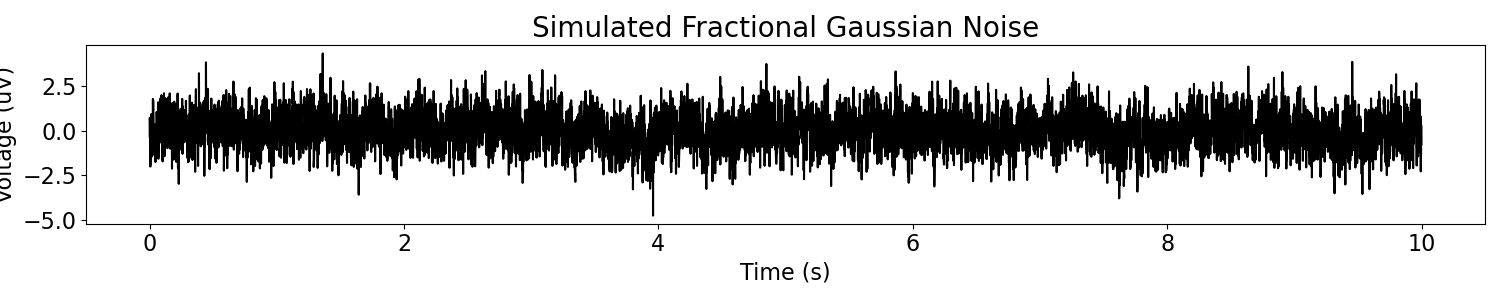
Fractional Gaussian Noise

To simulate a fractional gaussian noise signal, use the the sim_frac_gaussian_noise() function.

# Simulate fractional gaussian noise signal
gn_ap = sim_frac_gaussian_noise(n_seconds, fs, exponent=-.5)

# Plot the simulated data, in the time domain
plot_time_series(times, gn_ap, title='Simulated Fractional Gaussian Noise')

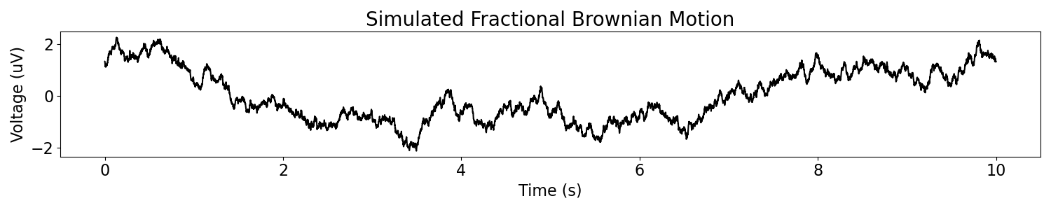
Fractional Brownian Motion

To simulate a fractional brownian motion signal, use the sim_frac_brownian_motion() function.

# Simulate fractional brownian motion signal
bm_ap = sim_frac_brownian_motion(n_seconds, fs, exponent=-2)

# Plot the simulated data, in the time domain
plot_time_series(times, bm_ap, title='Simulated Fractional Brownian Motion')