Spectral Domain Analysis: Variance

Apply spectral domain analyses, calculating variance measures.

This tutorial primarily covers the neurodsp.spectral.variance module.

Overview

This tutorial covers computing and displaying a spectral histogram, and computing the spectral coefficient of variation (SCV).

# Import spectral variance functions
from neurodsp.spectral import compute_spectral_hist, compute_scv, compute_scv_rs

# Import function to compute power spectra
from neurodsp.spectral import compute_spectrum

# Import utilities for loading and plotting data
from neurodsp.utils import create_times
from neurodsp.utils.download import load_ndsp_data
from neurodsp.plts.time_series import plot_time_series
from neurodsp.plts.spectral import (plot_spectral_hist, plot_scv,
                                    plot_scv_rs_lines, plot_scv_rs_matrix)

Load example neural signal

First, we load the sample data, which is a segment of rat hippocampal LFP taken from the publicly available database CRCNS (specifically, from the ‘hc2’ dataset).

Relevant publication: Mizuseki et al, 2012, Nature Neuro

# Download, if needed, and load example data files
sig = load_ndsp_data('sample_data_2.npy', folder='data')

# Set sampling rate, and create a times vector for plotting
fs = 1000
times = create_times(len(sig)/fs, fs)

# Plot the loaded signal
plot_time_series(times, sig, xlim=[0, 3])

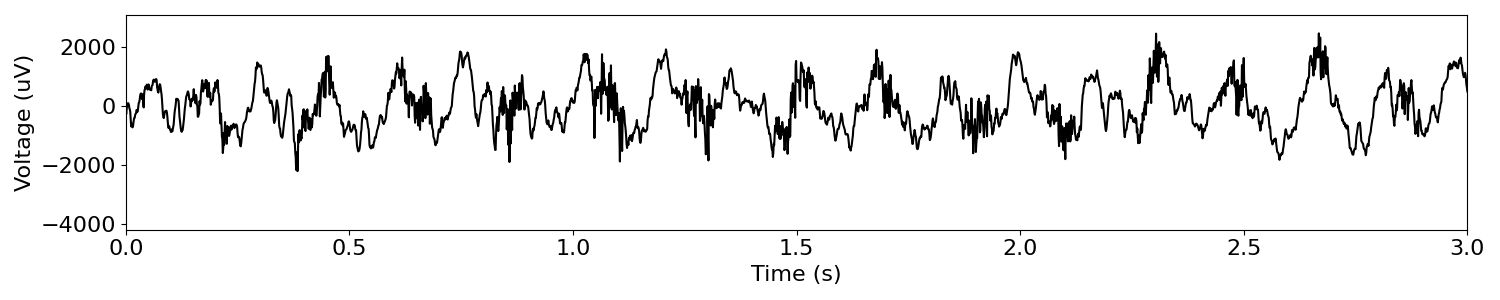
Plotting the data, we observe a strong theta oscillation (~6-8 Hz).

Spectral histogram

First, let’s look at computing spectral histograms, with compute_spectral_hist().

The PSD is an estimate of the central tendency (mean/median) of the signal’s power at each frequency, with the assumption that the signal is relatively stationary and that the variance around the mean comes from various forms of noise.

However, in physiological data, we may be interested in visualizing the distribution of power values around the mean at each frequency, as estimated in sequential slices of short-time Fourier transform (STFT), since it may reveal non-stationarities in the data or particular frequencies that are not like the rest. Here, we simply bin the log-power values across time, in a histogram, to observe the noise distribution at each frequency.

# Calculate the spectral histogram
freqs, bins, spect_hist = compute_spectral_hist(sig, fs, nbins=50, f_range=(0, 80),
                                                cut_pct=(0.1, 99.9))

# Calculate a power spectrum, with median Welch
freq_med, psd_med = compute_spectrum(sig, fs, method='welch',
                                     avg_type='median', nperseg=fs*2)

# Plot the spectral histogram
plot_spectral_hist(freqs, bins, spect_hist, freq_med, psd_med)

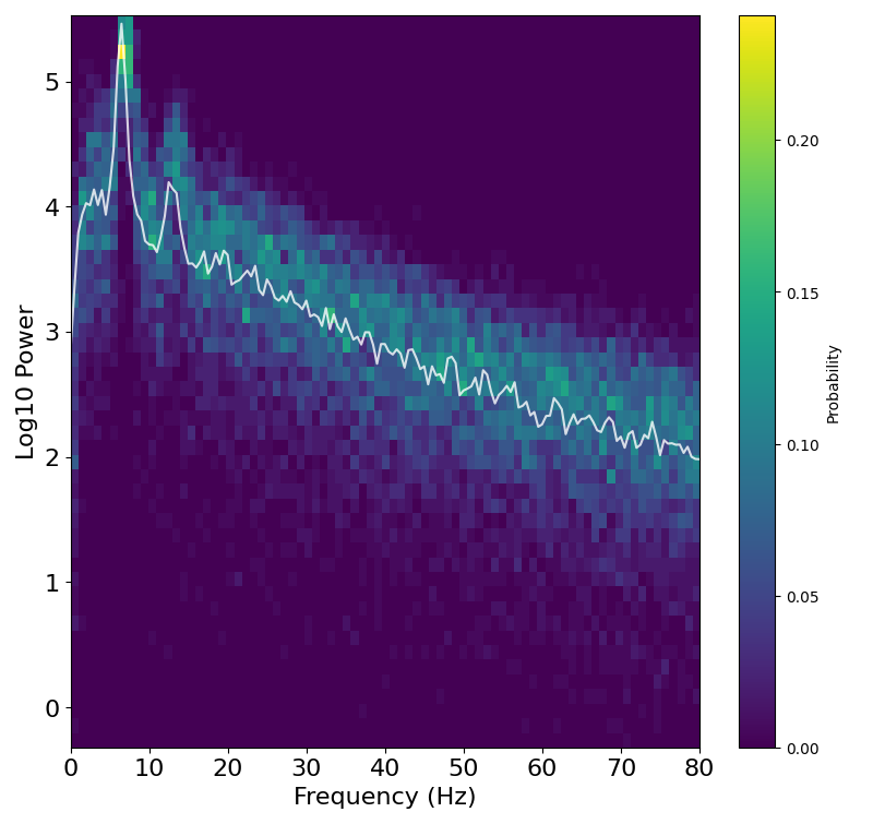
Notice in the plot that not only is theta power higher overall (shifted up), it also has lower variance around its mean.

Spectral Coefficient of Variation (SCV)

Next, let’s look at computing the spectral coefficient of variation, with compute_scv().

As noted above, the range of log-power values in the theta frequency range is lower compared to other frequencies, while that of 30-100Hz appear to be quite constant across the entire frequency axis (homoscedasticity).

To quantify that, we compute the coefficient of variation (standard deviation/mean) as a normalized estimate of variance.

# Calculate SCV
freqs, scv = compute_scv(sig, fs, nperseg=int(fs), noverlap=0)

There is also a plotting function for SCV, plot_scv().

# Plot the SCV
plot_scv(freqs, scv)

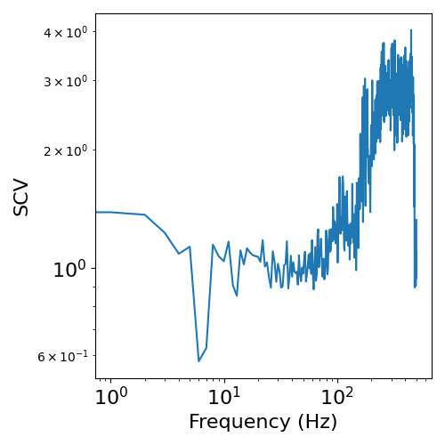
As shown above, SCV calculated from the entire segment of data is quite noisy due to the single estimate of mean and standard deviation.

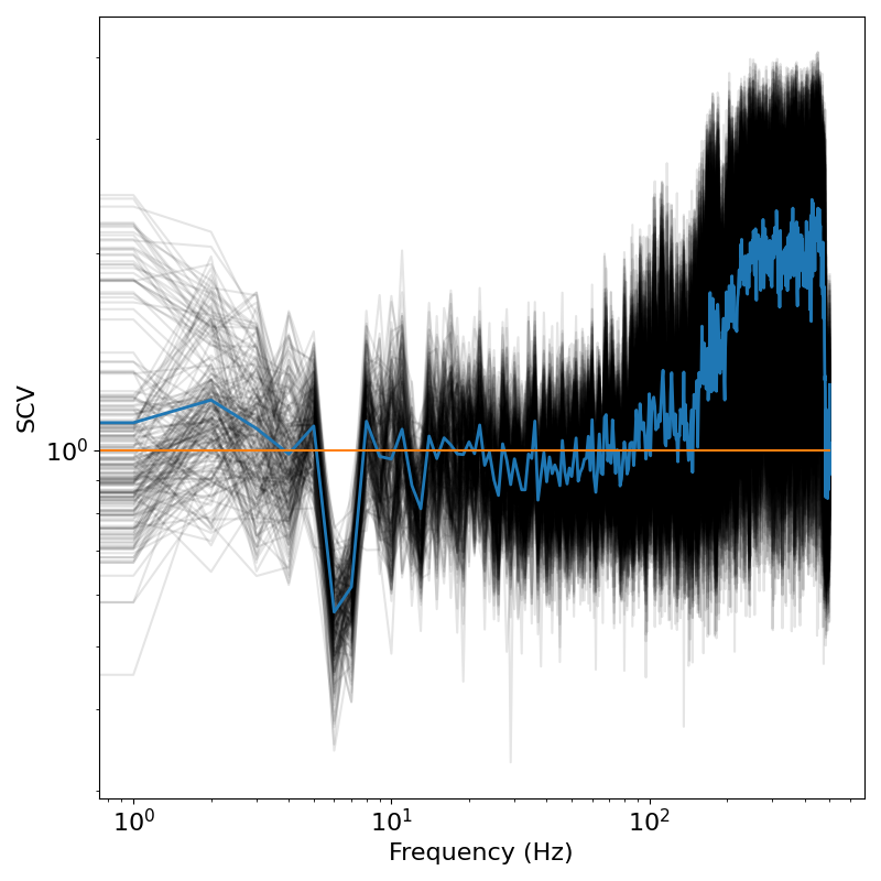
To overcome this, we can compute a bootstrap-resampled estimate of SCV, by randomly drawing slices from the non-overlapping spectrogram and taking their average.

The resampled spectral coefficient of variation can be computed with compute_scv_rs().

# Calculate SCV with the resampling method
freqs, t_inds, scv_rs = compute_scv_rs(sig, fs, nperseg=fs, method='bootstrap',
                                       rs_params=(20, 200))

You can plot the resampled SCV, as lines, with plot_scv_rs_lines().

# Plot the SCV, from the resampling method
plot_scv_rs_lines(freqs, scv_rs)

Another way to compute the resampled SCV is via a sliding window approach, essentially smoothing over consecutive slices of the spectrogram to compute the mean and standard deviation estimates.

# Calculate SCV with the resampling method
freqs, t_inds, scv_rs = compute_scv_rs(sig, fs, method='rolling', rs_params=(10, 2))

You can plot the resampled SCV, as a matrix, with plot_scv_rs_matrix().

# Plot the SCV, from the resampling method
plot_scv_rs_matrix(freqs, t_inds, scv_rs)

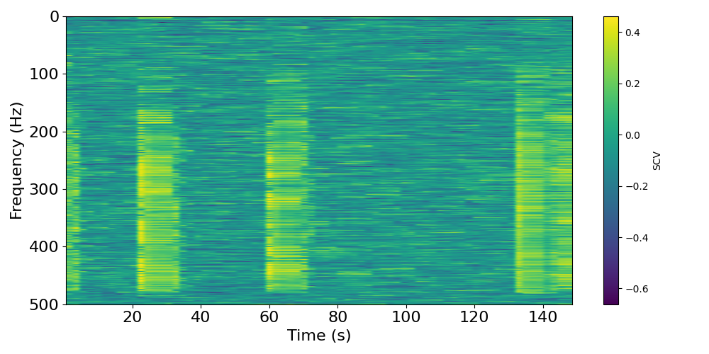
In the plot below, we see that the theta band (~7Hz) consistently has CV of less than 1 (negative in log10).